Unit 2 - Supply and Demand
Printable Cheat Sheets for Units 1–5
Single-page PDFs for Units 1-5. The full unit experience for Unit 6 stays on this cheat sheet page.
Download PDF Cheat SheetsTable of Contents
Built into this unit
Flashcards
94 cards mix graphs, formulas, and key terms. Shuffle blends every type so you drill the whole unit—not just one format.
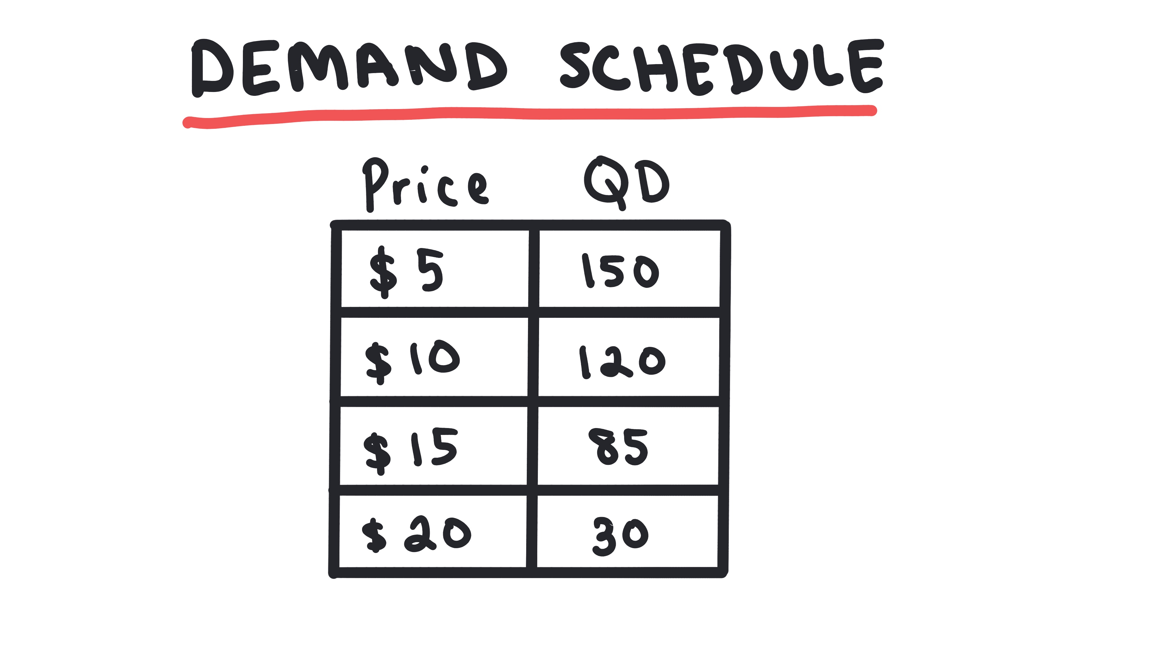
2.1 - Demand
Demand
Learn about the law of demand, demand curves, and demand schedules.
Key Terms & Definitions
Demand
The relationship between the price of a good or service and the quantity consumers are willing and able to purchase at various prices during a specific time period.
- •Demand represents willingness AND ability to pay
- •Demand is always downward sloping (Law of Demand)
- •Demand can shift due to non-price factors
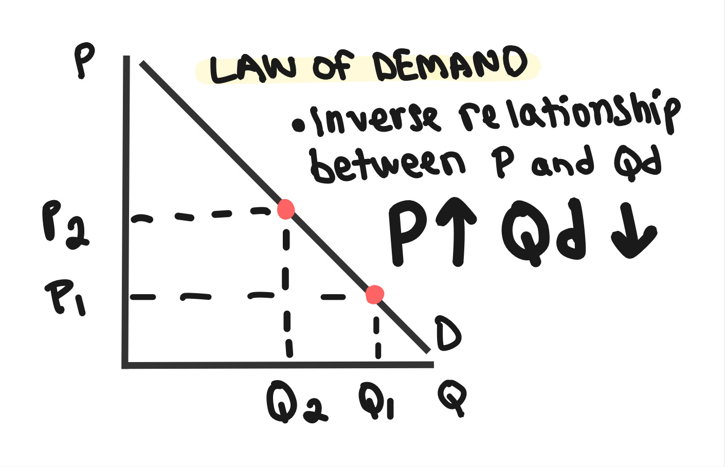
Law of Demand
The principle that, as the price of a good or service increases, the quantity demanded will decrease, and vice versa.
- •Price and quantity demanded have an inverse relationship
- •The demand curve always slopes downward from left to right
- •Two main reasons for the law of demand: substitution effect and income effect
Substitution Effect
When the price of a good increases, consumers substitute away from it and purchase relatively cheaper goods instead, decreasing the quantity demanded.
- •Example: If the price of chicken increases, consumers buy less chicken and more beef (substitute)
- •Works in reverse as well: if the price of a good decreases, consumers buy more of it and less of relatively more expensive goods
Income Effect
When the price of a good decreases, consumers' real purchasing power increases, allowing them to buy more of the good (and other goods) with the same nominal income.
- •Example: If I have 5.
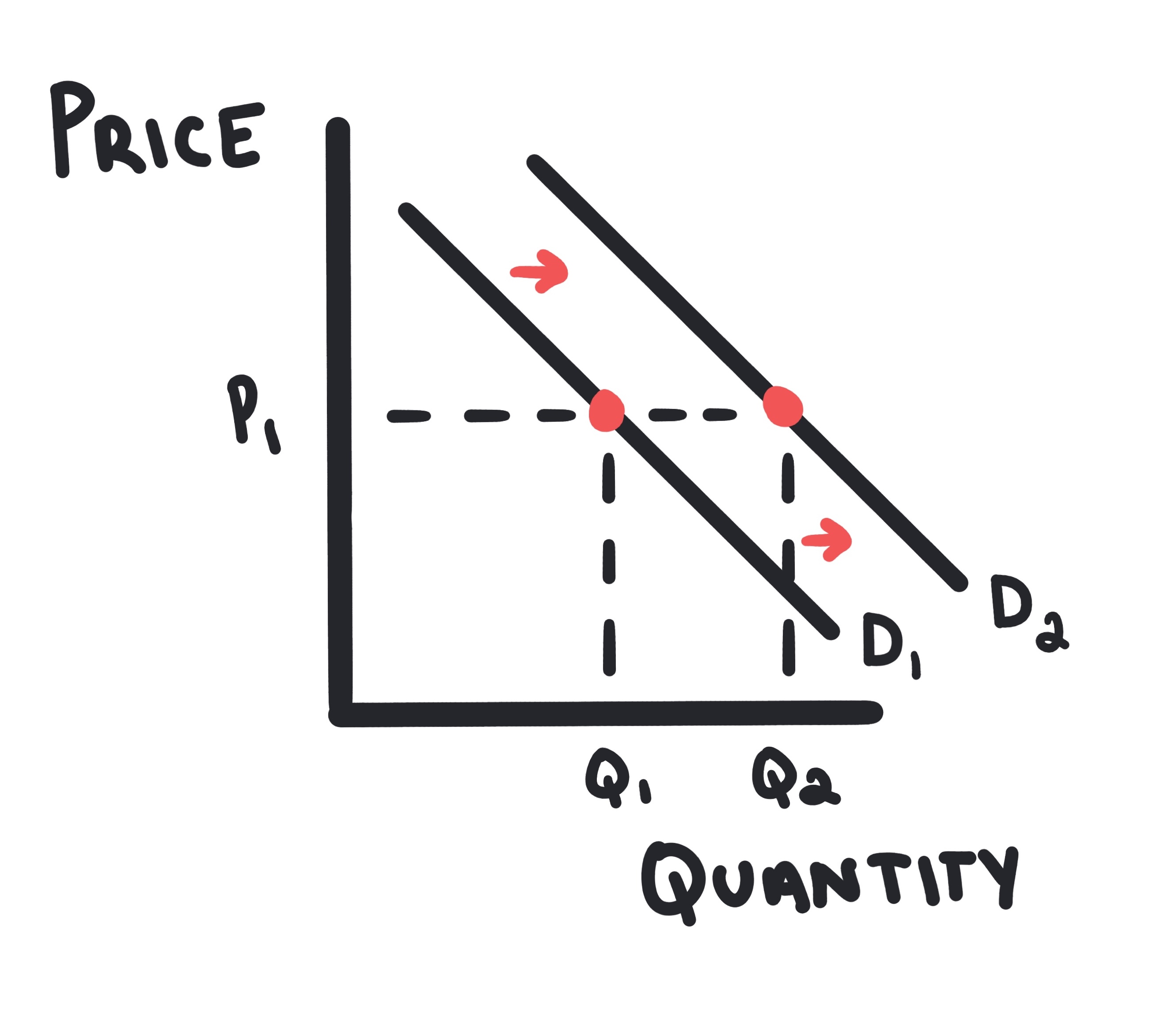
Determinants of Demand
Factors other than price that shift the demand curve.
- •Tastes and Preferences: Fidget spinners are no longer cool, so demand for them decreases.
- •Income: As a country becomes more wealthy, demand for luxury goods increases.
- •Prices of Related Goods: If Apple Music increases their price, demand for Spotify increases.
- •Number of Buyers: If more people move to Miami, demand for apartments in Miami increases.
- •Expectations: If people expect the price of gasoline to increase next week, they will buy more gasoline this week.
Normal Good
A good for which demand increases as consumer income rises, and demand decreases as consumer income falls (positive income elasticity).
- •Examples include most goods: cars, electronics, clothing
- •Has positive income elasticity of demand
- •Demand curve shifts right when income increases
- •Demand curve shifts left when income decreases
Inferior Good
A good for which demand decreases as consumer income rises, and demand increases as consumer income falls (negative income elasticity).
- •Examples include ramen noodles, used cars, public transportation
- •Has negative income elasticity of demand
- •Demand curve shifts left when income increases
- •Demand curve shifts right when income decreases
Substitutes
Two goods for which an increase in the price of one leads to an increase in the demand for the other (positive cross-price elasticity).
- •Examples: Coke and Pepsi, butter and margarine
- •Have positive cross-price elasticity of demand
- •Price increase of one shifts demand for the other right
- •Consumers can easily switch between them
Complements
Two goods for which an increase in the price of one leads to a decrease in the demand for the other (negative cross-price elasticity). Goods often consumed together.
- •Examples: peanut butter and jelly, cars and gasoline
- •Have negative cross-price elasticity of demand
- •Price increase of one shifts demand for the other left
- •Goods are consumed together as a bundle
Whiteboards
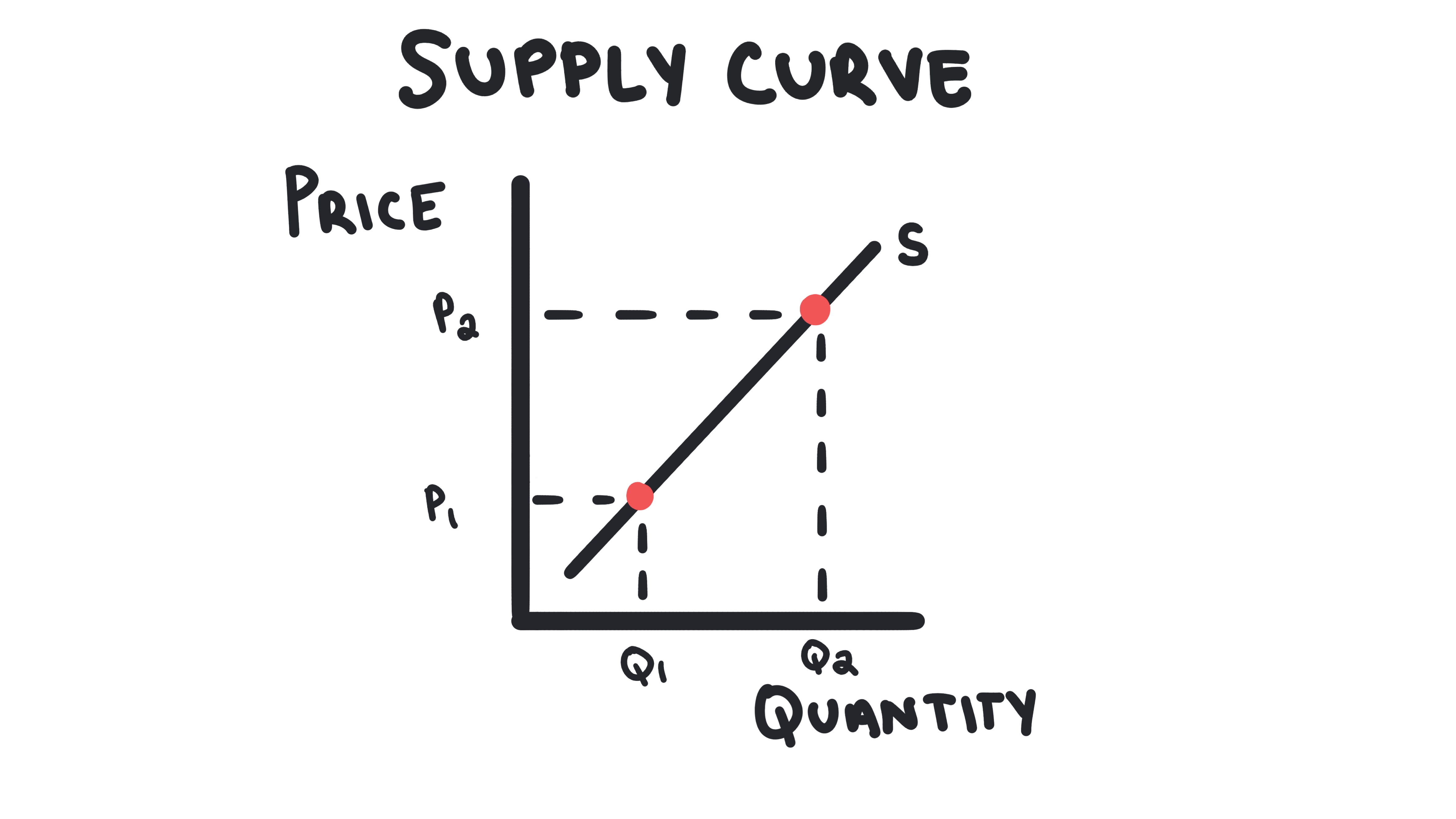
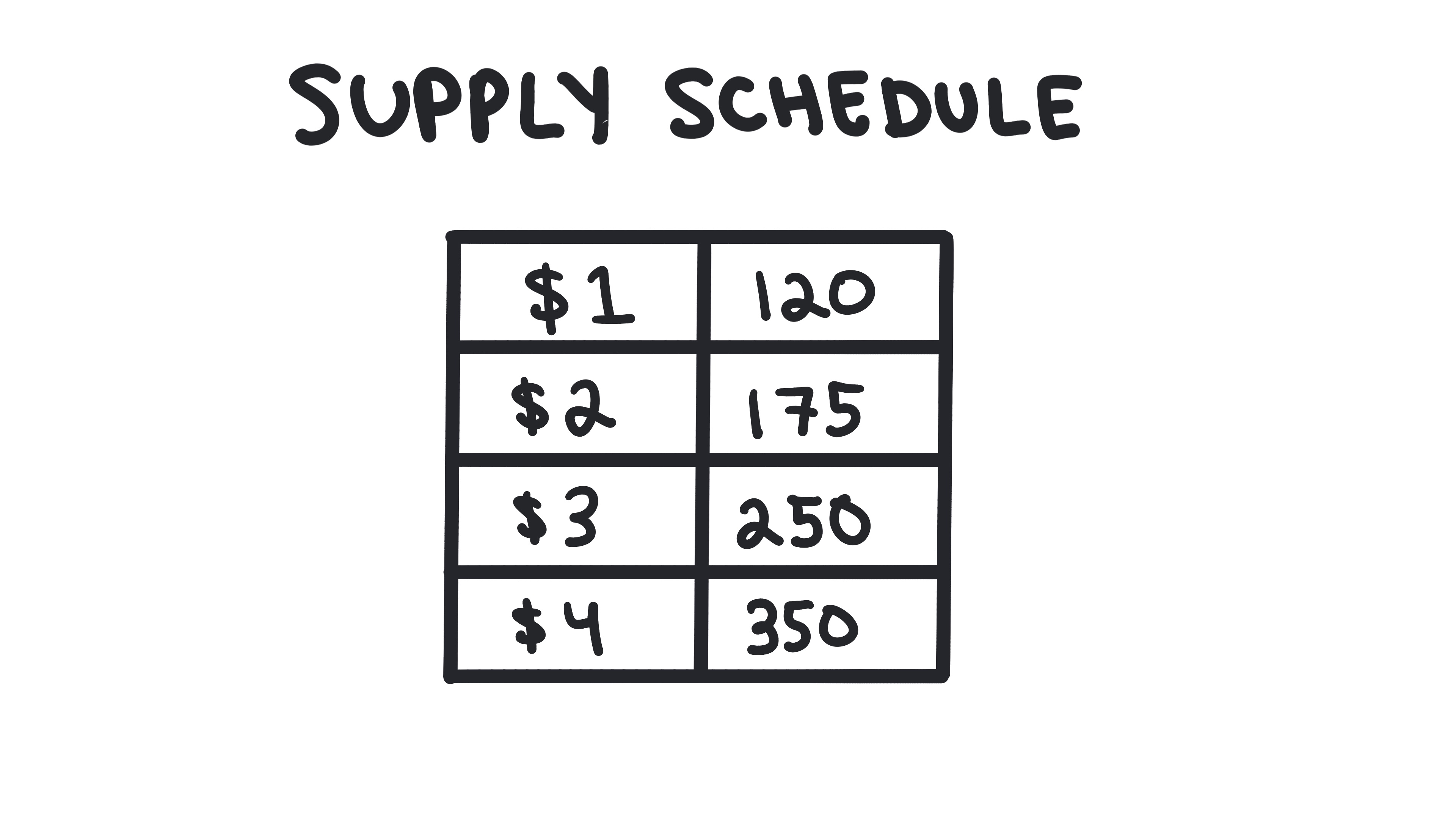
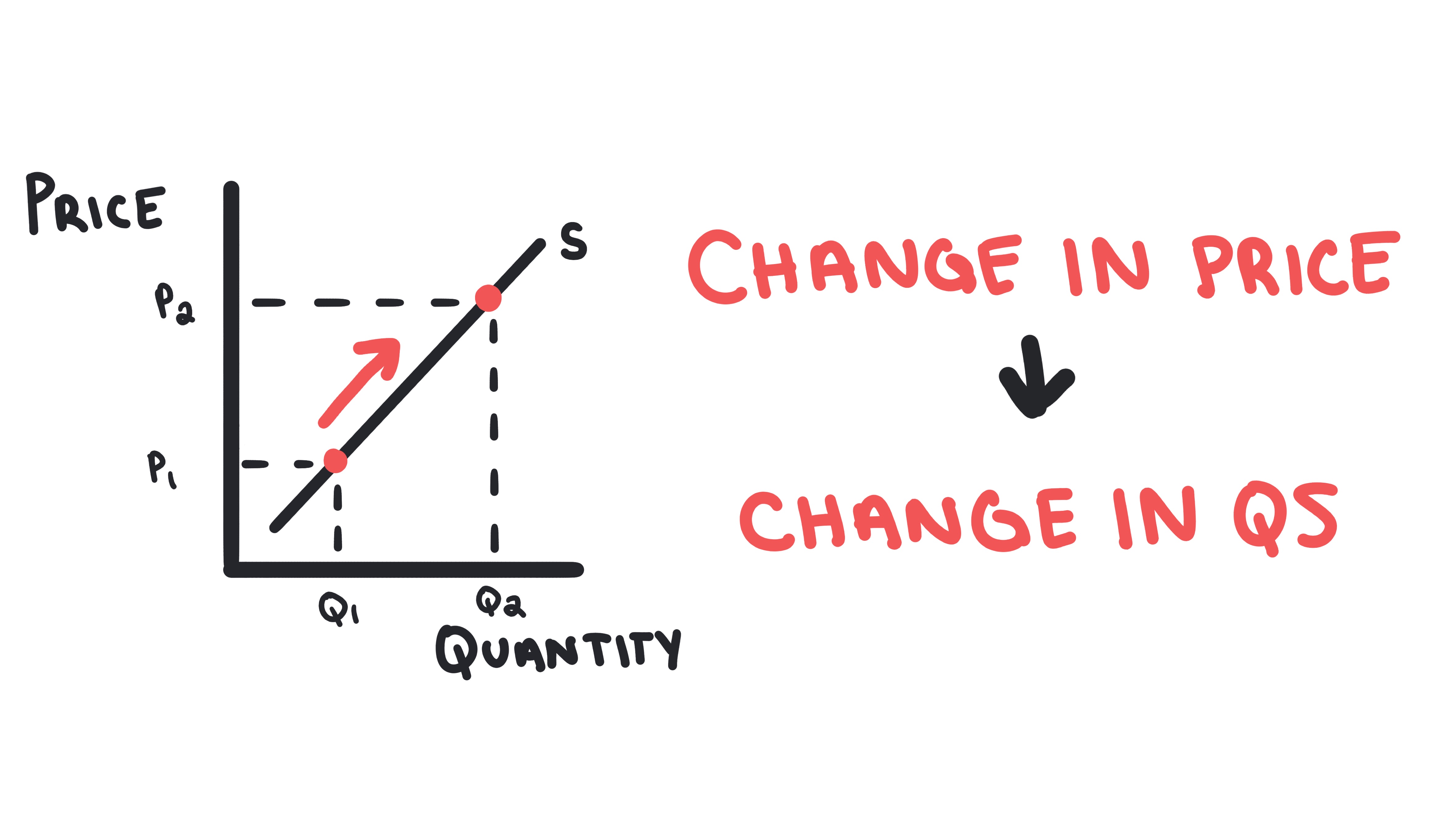
2.2 - Supply
Key Terms & Definitions
Supply
The relationship between the price of a good or service and the quantity producers are willing and able to sell at various prices during a specific time period, ceteris paribus.
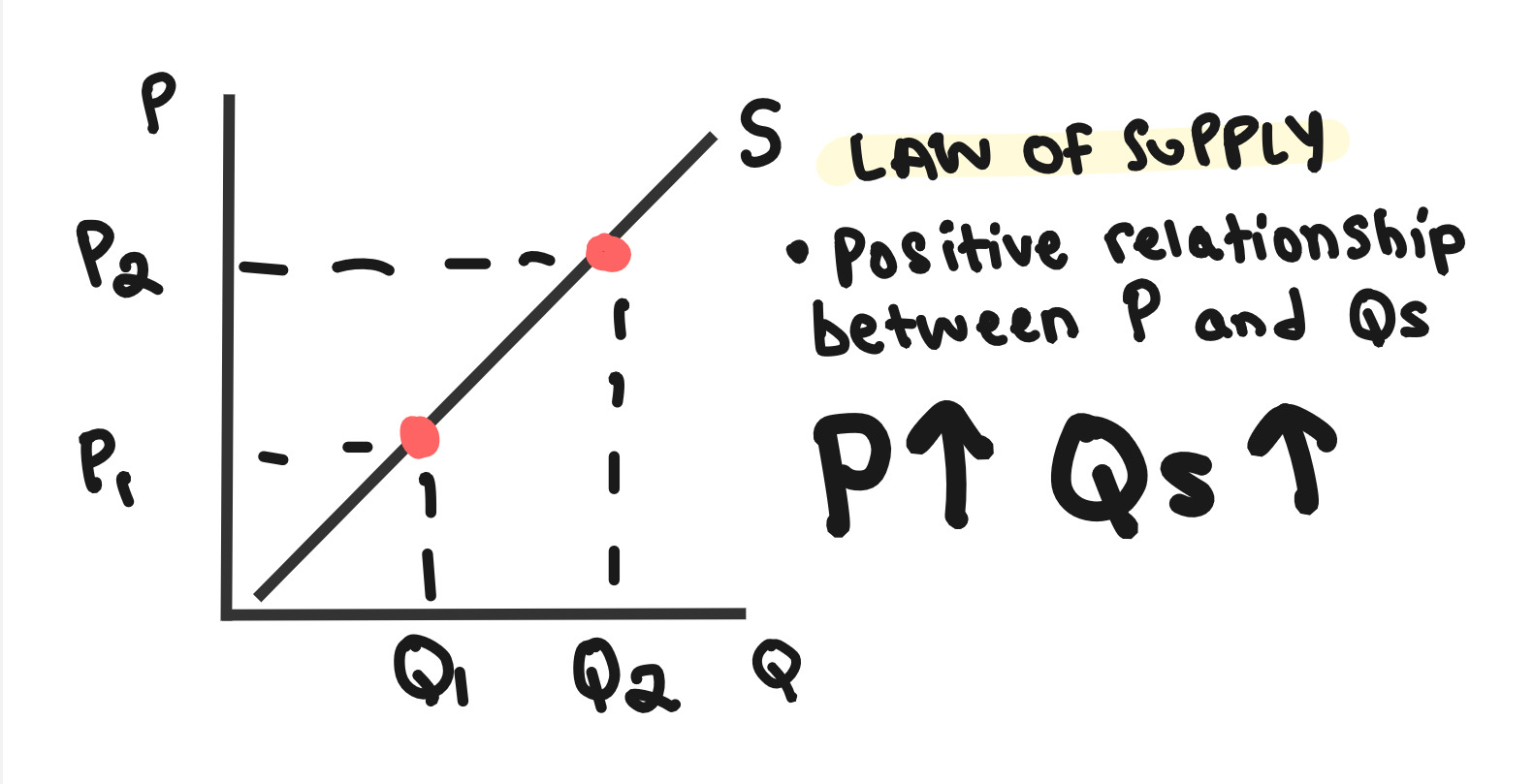
Law of Supply
The principle that, as the price of a good or service increases, the quantity supplied will increase, and vice versa.
- •Price and quantity supplied have a direct relationship
- •The supply curve always slopes upward
- •Two main reasons for the law of supply: profit motive and opportunity cost
Determinants of Supply
Factors other than price that shift the supply curve.
- •Resource Prices: Higher input costs shift supply left
- •Technology: Better technology shifts supply right
- •Number of Sellers: More sellers shifts supply right
- •Government Actions: Taxes shift supply left, subsidies shift right
Resource/Input Prices
The cost of factors of production (land, labor, capital, entrepreneurship) used to produce goods and services. Changes in these costs shift the supply curve.
- •Higher input costs shift supply curve left (decrease supply)
- •Lower input costs shift supply curve right (increase supply)
- •Examples: If I produce wooden tables, and the price of wood increases, I can produce fewer tables with the same amount of money.
Technology
The methods, processes, and techniques used to produce goods and services. Improvements in technology can increase productivity and shift the supply curve.
- •Better technology shifts supply curve right (increase supply)
- •Increases productivity and reduces production costs
- •Examples: New improved fertilizer allows farmers to produce more crops with the same amount of land and labor.
Prices of Other Goods
The prices of alternative goods that producers could produce instead. Changes in these prices can affect the supply of the current good.
- •Higher prices of alternatives shift supply left (decrease supply)
- •Lower prices of alternatives shift supply right (increase supply)
- •Producers switch to more profitable alternatives
- •Examples: If the price of durian increase, farmers will produce more durian and less other fruits.
Number of Sellers
The quantity of firms or producers in a market. Changes in the number of sellers directly affect the total supply in the market.
- •More sellers shift supply curve right (increase supply)
- •Fewer sellers shift supply curve left (decrease supply)
- •Each seller contributes to total market supply
- •Examples: new firms entering, existing firms exiting
Expectations
Producers' beliefs about future market conditions, including prices, costs, and demand. These expectations can influence current supply decisions.
- •Expected higher future prices shift supply left (decrease current supply)
- •Expected lower future prices shift supply right (increase current supply)
- •Producers may hold inventory or rush to sell
- •Examples: If sellers of gold expect the price of gold to increase, they will sell less today and wait to sell more at the higher future price.
Government Actions
Policies and regulations implemented by government that affect production costs or incentives, including taxes, subsidies, regulations, and trade policies.
- •Taxes shift supply curve left (decrease supply)
- •Subsidies shift supply curve right (increase supply)
- •Regulations can increase costs and decrease supply
- •Examples: excise taxes, production subsidies, environmental regulations
Subsidy
A government payment to producers (or consumers) that reduces production costs, encouraging increased supply.
- •Shifts the supply curve to the right (increases supply)
- •Lowers production costs for firms
- •Example: Government gives subsidy to electric car company, allowing them to produce more electric cars at each price level
Whiteboards
2.3 - Price Elasticity of Demand
Price Elasticity of Demand
Learn about price elasticity of demand, how to calculate it, and factors that affect elasticity.
Key Terms & Definitions
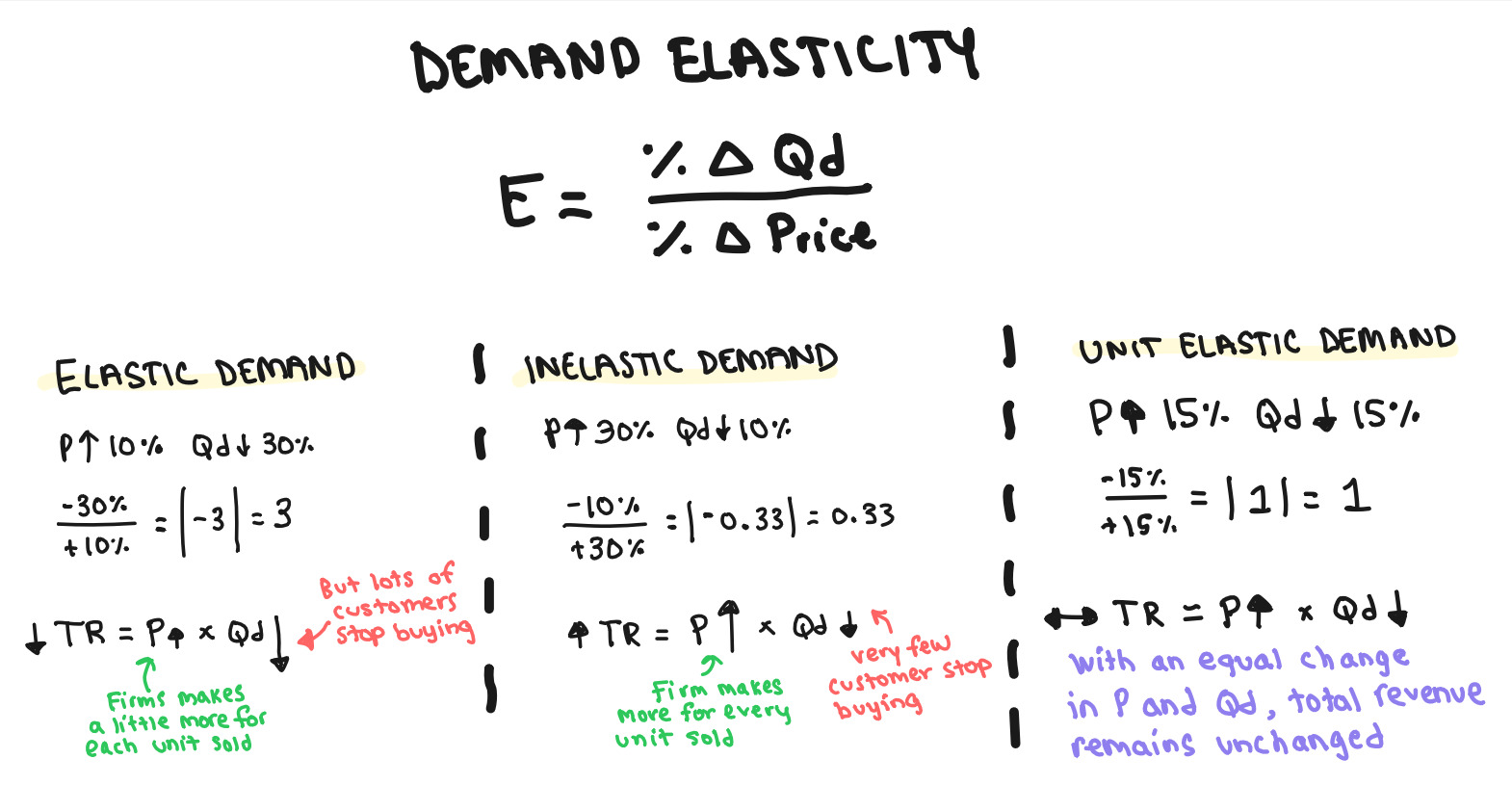
Price Elasticity of Demand (PED)
A measure of how responsive the quantity demanded of a good is to a change in its price. Calculated as: PED = (% change in Qd) / (% change in P).
- •The law of demand tell us that when price increases, people buy less. Price elasticity of demand tells us how much less they buy.
Elastic Demand
When the percentage change in quantity demanded is greater than the percentage change in price (|PED| > 1). Consumers are relatively responsive to price changes.
- •|PED| > 1 (absolute value greater than 1)
- •Consumers are very responsive to price changes
- •Examples: luxury goods, goods with many substitutes
- •Price increase leads to larger decrease in quantity demanded
Inelastic Demand
When the percentage change in quantity demanded is less than the percentage change in price (|PED| < 1). Consumers are relatively unresponsive to price changes.
- •|PED| < 1 (absolute value less than 1)
- •Consumers are not very responsive to price changes
- •Examples: necessities, goods with few substitutes
- •Price increase leads to smaller decrease in quantity demanded
Unit Elastic Demand
When the percentage change in quantity demanded is equal to the percentage change in price (|PED| = 1).
- •|PED| = 1 (absolute value equals 1)
- •Percentage change in Qd equals percentage change in P
- •Total revenue remains constant when price changes
Perfectly Inelastic Demand
When the quantity demanded does not change regardless of the price (PED = 0). The demand curve is vertical.
- •PED = 0 (no change in quantity when price changes)
- •Demand curve is perfectly vertical
- •Examples: life-saving medications, essential goods
- •Consumers will pay any price for the good
Perfectly Elastic Demand
When any increase in price causes the quantity demanded to drop to zero (|PED| = ∞). The demand curve is horizontal.
- •|PED| = ∞ (infinite elasticity)
- •Demand curve is perfectly horizontal
- •Examples: perfectly competitive markets, identical goods
- •Any price increase causes quantity demanded to fall to zero
Total Revenue Test
A method to determine price elasticity of demand by examining how total revenue (TR = P × Q) changes when price changes. If P and TR move opposite, demand is elastic. If P and TR move together, demand is inelastic. If TR is constant, demand is unit elastic.
- •P and TR move in opposite directions = elastic demand
- •P and TR move in same direction = inelastic demand
- •TR stays constant = unit elastic demand
- •Useful when elasticity formula is not available
Whiteboards
2.4 - Price Elasticity of Supply
Key Terms & Definitions
Price Elasticity of Supply (PES)
A measure of how responsive the quantity supplied of a good is to a change in its price. Calculated as: PES = (% change in Qs) / (% change in P).
- •Measures producer responsiveness to price changes
- •PES = %ΔQs / %ΔP (no absolute value needed)
- •Always positive due to Law of Supply
- •Depends on time period and production flexibility
Elastic Supply
When the percentage change in quantity supplied is greater than the percentage change in price (PES > 1). Producers are relatively responsive to price changes.
- •PES > 1 (greater than 1)
- •Examples: goods with flexible production, long time periods
- •Price increase leads to larger increase in quantity supplied
Inelastic Supply
When the percentage change in quantity supplied is less than the percentage change in price (PES < 1). Producers are relatively unresponsive to price changes.
- •PES < 1 (less than 1)
- •Examples: goods with fixed production, short time periods
- •Price increase leads to smaller increase in quantity supplied
2.5 - Other Elasticities
Other Elasticities
Learn about income elasticity, cross-price elasticity, and other measures of elasticity.
Key Terms & Definitions
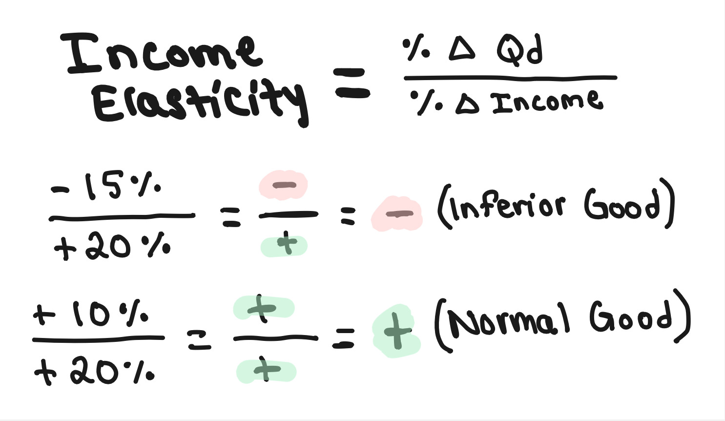
Normal Good
A good for which demand increases as consumer income rises, and demand decreases as consumer income falls (positive income elasticity).
- •Examples include most goods: cars, electronics, clothing
- •Has positive income elasticity of demand
- •Demand curve shifts right when income increases
- •Demand curve shifts left when income decreases
Inferior Good
A good for which demand decreases as consumer income rises, and demand increases as consumer income falls (negative income elasticity).
- •Examples include ramen noodles, used cars, public transportation
- •Has negative income elasticity of demand
- •Demand curve shifts left when income increases
- •Demand curve shifts right when income decreases
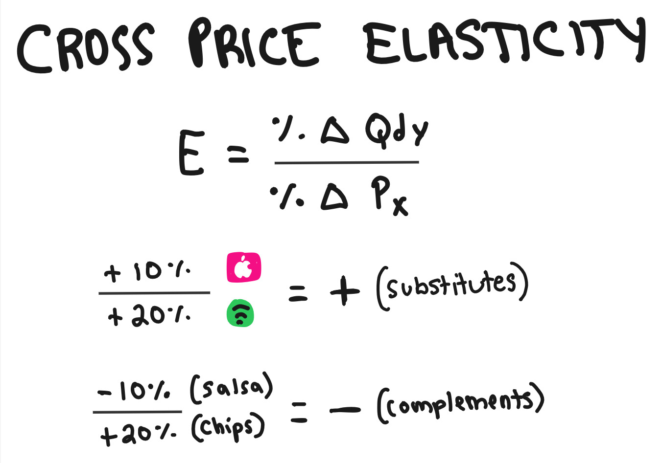
Substitutes
Two goods for which an increase in the price of one leads to an increase in the demand for the other (positive cross-price elasticity).
- •Examples: Coke and Pepsi, butter and margarine
- •Have positive cross-price elasticity of demand
- •Price increase of one shifts demand for the other right
- •Consumers can easily switch between them
Complements
Two goods for which an increase in the price of one leads to a decrease in the demand for the other (negative cross-price elasticity). Goods often consumed together.
- •Examples: peanut butter and jelly, cars and gasoline
- •Have negative cross-price elasticity of demand
- •Price increase of one shifts demand for the other left
- •Goods are consumed together as a bundle
Income Elasticity of Demand (YED)
A measure of how responsive the quantity demanded of a good is to a change in consumer income. Calculated as: YED = (% change in Qd) / (% change in Income).
- •YED > 0 → normal good (demand rises when income rises)
- •YED < 0 → inferior good (demand falls when income rises)
- •YED = 0 → quantity demanded does not change with income
Cross-Price Elasticity of Demand (XED)
A measure of how responsive the quantity demanded of one good is to a change in the price of another good. Calculated as: XED = (% change in Qd of Good A) / (% change in P of Good B).
- •XED > 0 → substitutes (higher price of B increases demand for A)
- •XED < 0 → complements (higher price of B decreases demand for A)
- •XED = 0 → unrelated goods (demand for A does not depend on the price of B)
Whiteboards
2.6 - Market Equilibrium and Consumer and Producer Surplus
Market Equilibrium and Consumer and Producer Surplus
Learn about market equilibrium, consumer surplus, and producer surplus.
Key Terms & Definitions
Market Equilibrium
The state where the quantity demanded equals the quantity supplied at a specific price.
- •Occurs where demand and supply curves intersect
- •No shortage or surplus at equilibrium
- •Market automatically moves toward equilibrium
Equilibrium Price
The price at which quantity demanded equals quantity supplied in a market. Also known as the market-clearing price (P* or Pe).
- •Occurs where demand and supply curves intersect
Equilibrium Quantity
The quantity of a good or service bought and sold at the equilibrium price (Q* or Qe).
- •Occurs where demand and supply curves intersect
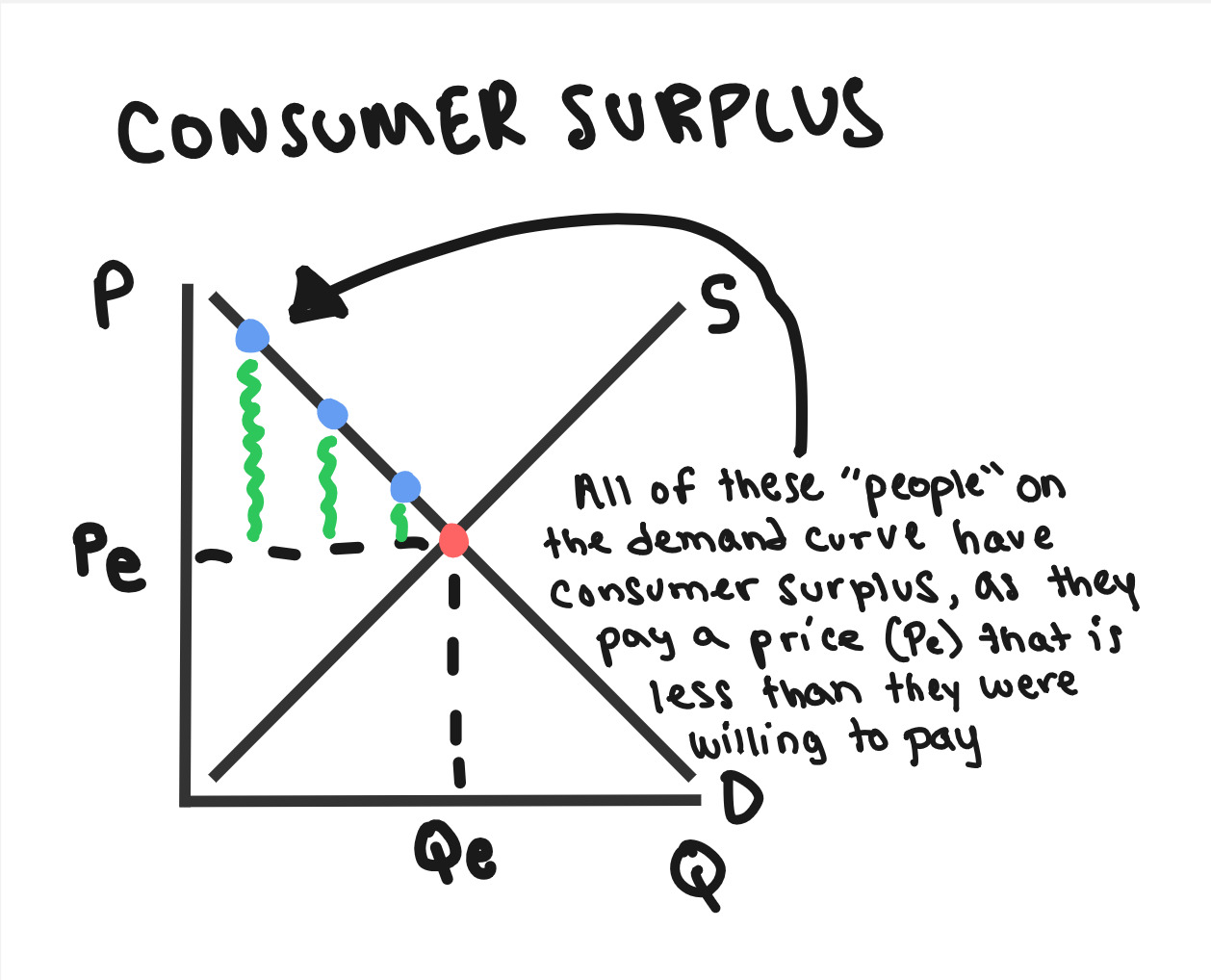
Consumer Surplus (CS)
The difference between the maximum price consumers are willing to pay for a unit of a good and the price they actually pay (market price). Represented graphically by the area below the demand curve and above the market price.
- •Area below demand curve and above market price
- •Measures consumer benefit from market transactions
- •Increases when price decreases
- •Decreases when price increases
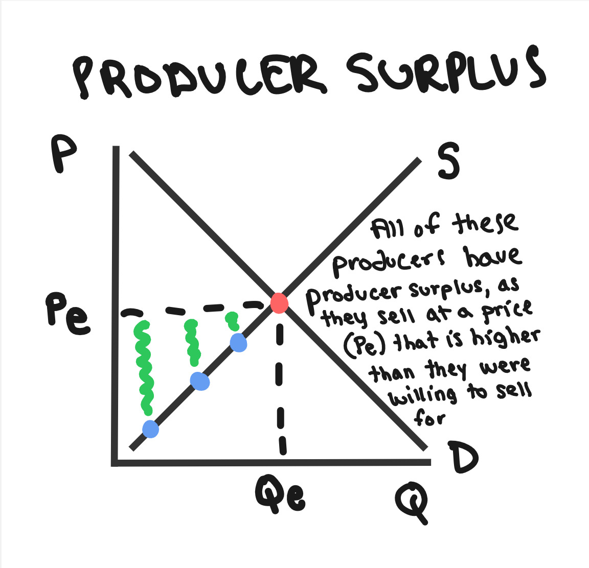
Producer Surplus (PS)
The difference between the price producers actually receive for a unit of a good (market price) and the minimum price they are willing to accept (marginal cost). Represented graphically by the area above the supply curve and below the market price.
- •Area above supply curve and below market price
- •Measures producer benefit from market transactions
- •Increases when price increases
- •Decreases when price decreases
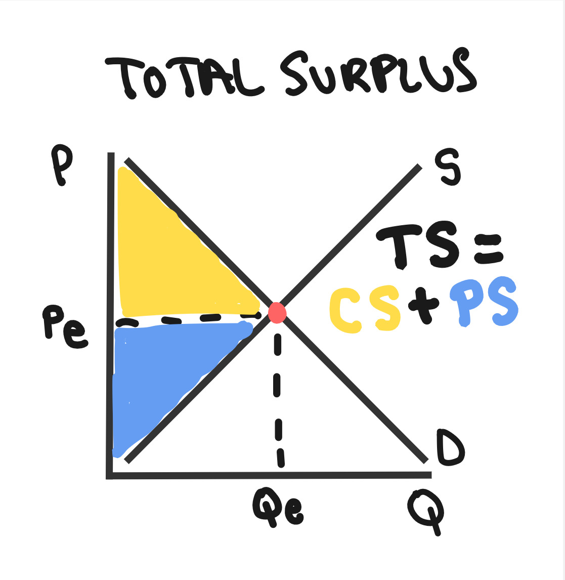
Total Surplus (TS)
The sum of consumer surplus and producer surplus (TS = CS + PS). It represents the total welfare or benefit to society from market transactions and is maximized at market equilibrium.
- •TS = CS + PS (sum of both surpluses)
- •Maximized at market equilibrium
- •Measures total welfare to society
- •Any market distortion reduces total surplus
Whiteboards
2.7 - Market Disequilibrium and Changes in Equilibrium
Market Disequilibrium and Changes in Equilibrium
Learn about market disequilibrium, shortages, surpluses, and how shifts in supply and demand change equilibrium.
Key Terms & Definitions
Market Equilibrium
The state where the quantity demanded equals the quantity supplied at a specific price.
- •Occurs where demand and supply curves intersect
- •No shortage or surplus at equilibrium
- •Market automatically moves toward equilibrium
Equilibrium Price
The price at which quantity demanded equals quantity supplied in a market. Also known as the market-clearing price (P* or Pe).
- •Occurs where demand and supply curves intersect
Equilibrium Quantity
The quantity of a good or service bought and sold at the equilibrium price (Q* or Qe).
- •Occurs where demand and supply curves intersect
Shortage
A situation where the quantity demanded (Qd) exceeds the quantity supplied (Qs) at the current price (Qd > Qs). Occurs when the price is below equilibrium.
- •Also called excess demand
- •Creates upward pressure on price
- •Some consumers cannot buy the good
- •Market will adjust toward equilibrium
Surplus
A situation where the quantity supplied (Qs) exceeds the quantity demanded (Qd) at the current price (Qs > Qd). Occurs when the price is above equilibrium.
- •Also called excess supply
- •Creates downward pressure on price
- •Some producers cannot sell their goods
- •Market will adjust toward equilibrium
Whiteboards

2.8 - The Effects of Government Intervention in Markets
The Effects of Government Intervention in Markets
Learn how government policies such as price controls and taxes affect markets.
Key Terms & Definitions
Shortage
A situation where the quantity demanded (Qd) exceeds the quantity supplied (Qs) at the current price (Qd > Qs). Occurs when the price is below equilibrium.
- •Also called excess demand
- •Creates upward pressure on price
- •Some consumers cannot buy the good
- •Market will adjust toward equilibrium
Surplus
A situation where the quantity supplied (Qs) exceeds the quantity demanded (Qd) at the current price (Qs > Qd). Occurs when the price is above equilibrium.
- •Also called excess supply
- •Creates downward pressure on price
- •Some producers cannot sell their goods
- •Market will adjust toward equilibrium
Total Surplus (TS)
The sum of consumer surplus and producer surplus (TS = CS + PS). It represents the total welfare or benefit to society from market transactions and is maximized at market equilibrium.
- •TS = CS + PS (sum of both surpluses)
- •Maximized at market equilibrium
- •Measures total welfare to society
- •Any market distortion reduces total surplus
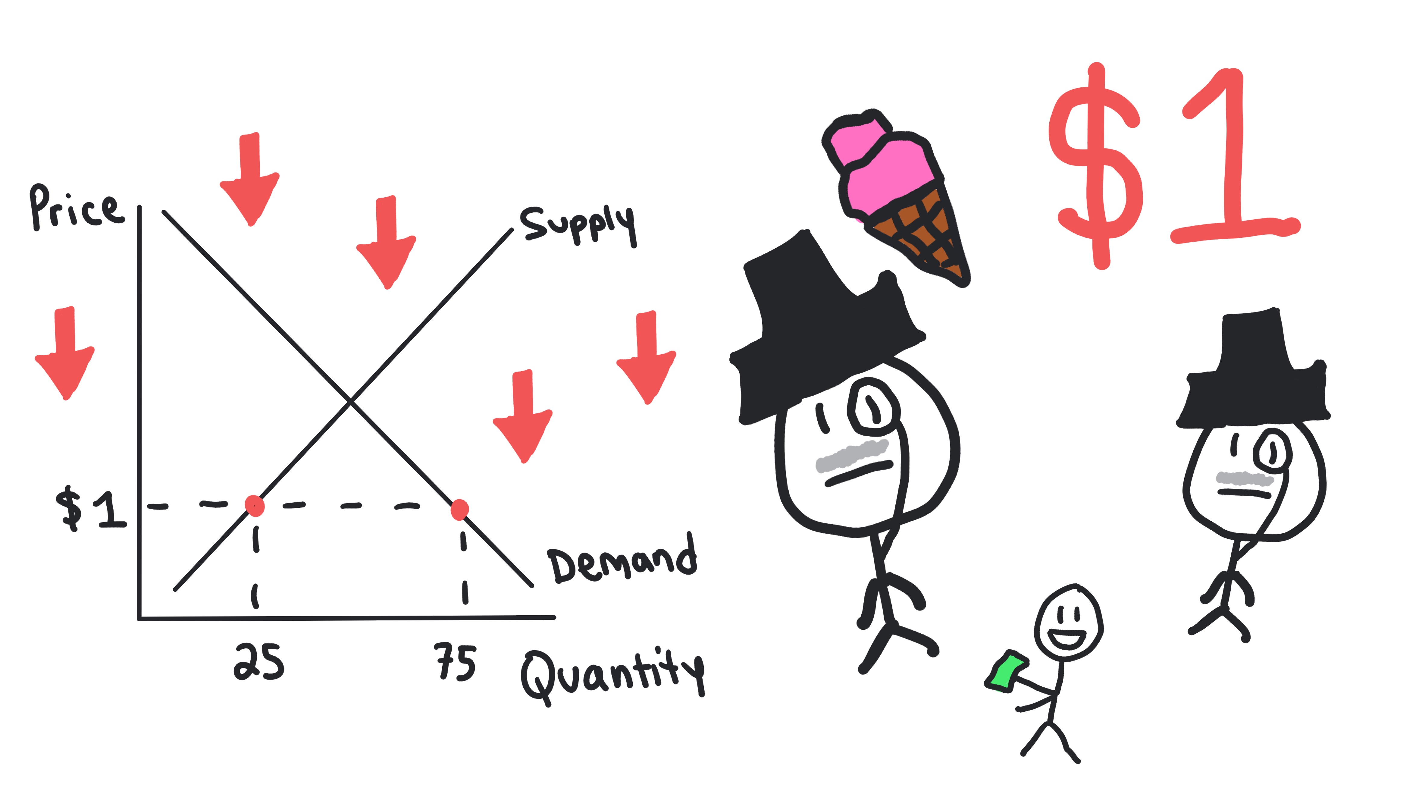
Price Ceiling
A legally established maximum price that can be charged for a good or service. To be binding (effective), it must be set below the equilibrium price, typically leading to a shortage (Qd > Qs).
- •Must be below equilibrium price to be binding
- •Creates shortage (excess demand)
- •Examples: rent controls, price caps on utilities
- •Reduces total surplus and creates deadweight loss
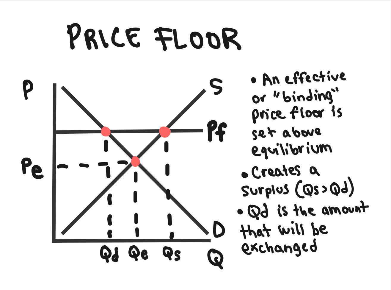
Price Floor
A legally established minimum price that can be charged for a good or service. To be binding (effective), it must be set above the equilibrium price, typically leading to a surplus (Qs > Qd).
- •Must be above equilibrium price to be binding
- •Creates surplus (excess supply)
- •Examples: minimum wage, agricultural price supports
- •Reduces total surplus and creates deadweight loss
Excise Tax
A per-unit tax levied on the production or sale of a specific good or service. It shifts the supply curve upward (or demand curve downward), increases the price buyers pay, decreases the price sellers receive, reduces the equilibrium quantity, and creates deadweight loss.
- •Per-unit tax on specific goods (not income tax)
- •Shifts supply curve up by amount of tax
- •Increases price buyers pay, decreases price sellers receive
- •Creates deadweight loss and reduces total surplus
Tax Incidence
The distribution of the burden of a tax between buyers and sellers. The incidence depends on the relative price elasticities of demand and supply; the more inelastic side bears a larger share of the tax burden.
- •More inelastic side bears larger tax burden
- •Inelastic demand = consumers pay more of tax
- •Inelastic supply = producers pay more of tax
- •Tax burden is independent of who legally pays the tax
Subsidy
A government payment to buyers or sellers, usually on a per-unit basis, intended to encourage production or consumption. It effectively lowers the cost for producers (shifting supply right) or the price for consumers (shifting demand right), increasing quantity and potentially creating deadweight loss if it pushes quantity beyond the efficient level.
- •Government payment to encourage production/consumption
- •Shifts supply curve right or demand curve right
- •Increases equilibrium quantity
- •Can create deadweight loss if over-subsidized
Deadweight Loss (DWL)
The loss of total surplus (combined consumer and producer surplus) that results from a market distortion, such as a tax, price control, or externality, which prevents the market from reaching the efficient equilibrium quantity.
- •Triangle area between supply and demand curves
- •Created by taxes, price controls, quotas, externalities
- •Represents value of mutually beneficial trades that don't occur
Whiteboards
2.9 - International Trade and Public Policy
International Trade and Public Policy
Learn about international trade, tariffs, and the effects of public policy on markets.
Key Terms & Definitions
Quota (Quantity Control)
An upper limit set by the government on the quantity of a good that can be bought or sold. Leads to inefficiencies such as deadweight loss and incentives for illegal activities.
- •Government limit on quantity bought/sold
- •Creates artificial scarcity and higher prices
- •Examples: fishing quotas, import quotas
- •Leads to deadweight loss and black market activity
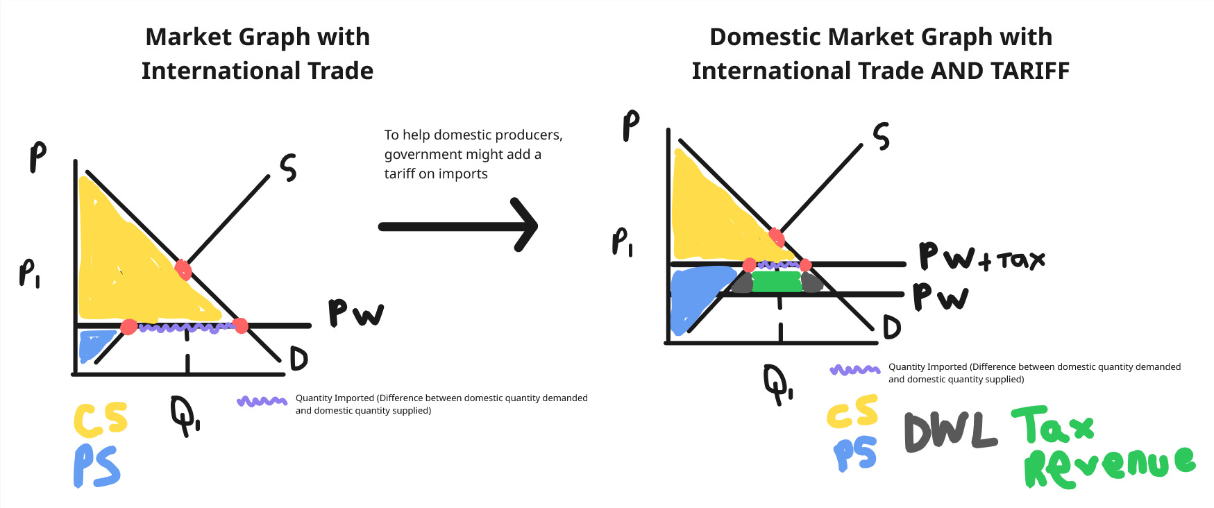
Tariff
A tax imposed by the government on imported goods, raising the price of imports and reducing the quantity imported.
- •Increases the price of imported goods
- •Reduces quantity imported
- •Shifts the supply curve for imports left (decreases supply)
- •Creates deadweight loss and reduces total surplus
- •Example: Government imposes tariff on imported steel, making foreign steel more expensive
Quantity Imported
The amount of a good that a country purchases from foreign producers. On a graph, it is the difference between domestic quantity demanded and domestic quantity supplied at the world price.
- •How to find on a graph: At the world price, find where the price line intersects the domestic demand curve (Qd) and where it intersects the domestic supply curve (Qs)
- •Quantity Imported = Qd - Qs (at the world price)
- •If Qd > Qs at world price, the country imports the difference
- •If Qd < Qs at world price, the country exports instead (negative imports)
- •Example: If domestic demand is 100 units and domestic supply is 60 units at world price, quantity imported = 40 units
Whiteboards