Unit 3 - National Income and Price Determination
Printable Cheat Sheets for Every Unit
Everything you need to ace your exam, all on a single page.
Download PDF Cheat SheetsTable of Contents
Built into this unit
Flashcards
73 cards mix graphs, formulas, and key terms. Shuffle blends every type so you drill the whole unit—not just one format.

3.1 - Aggregate Demand (AD)
Aggregate Demand
Learn about the components of aggregate demand, the relationship between aggregate demand and the price level, and the impact of changes in aggregate demand on the economy.
Key Terms & Definitions
Aggregate
A word that simply means "total" or "combined." In this unit, it means we are looking at the demand for all goods and services in an entire economy, not just one product.
Price Level
The overall or average level of prices in an economy. It is represented on the vertical axis of the AD-AS graph.
Aggregate Demand (AD)
The total demand for all goods and services in an economy. The AD curve shows the amount of goods and services that households, businesses, the government, and foreign customers are willing to buy at different price levels.
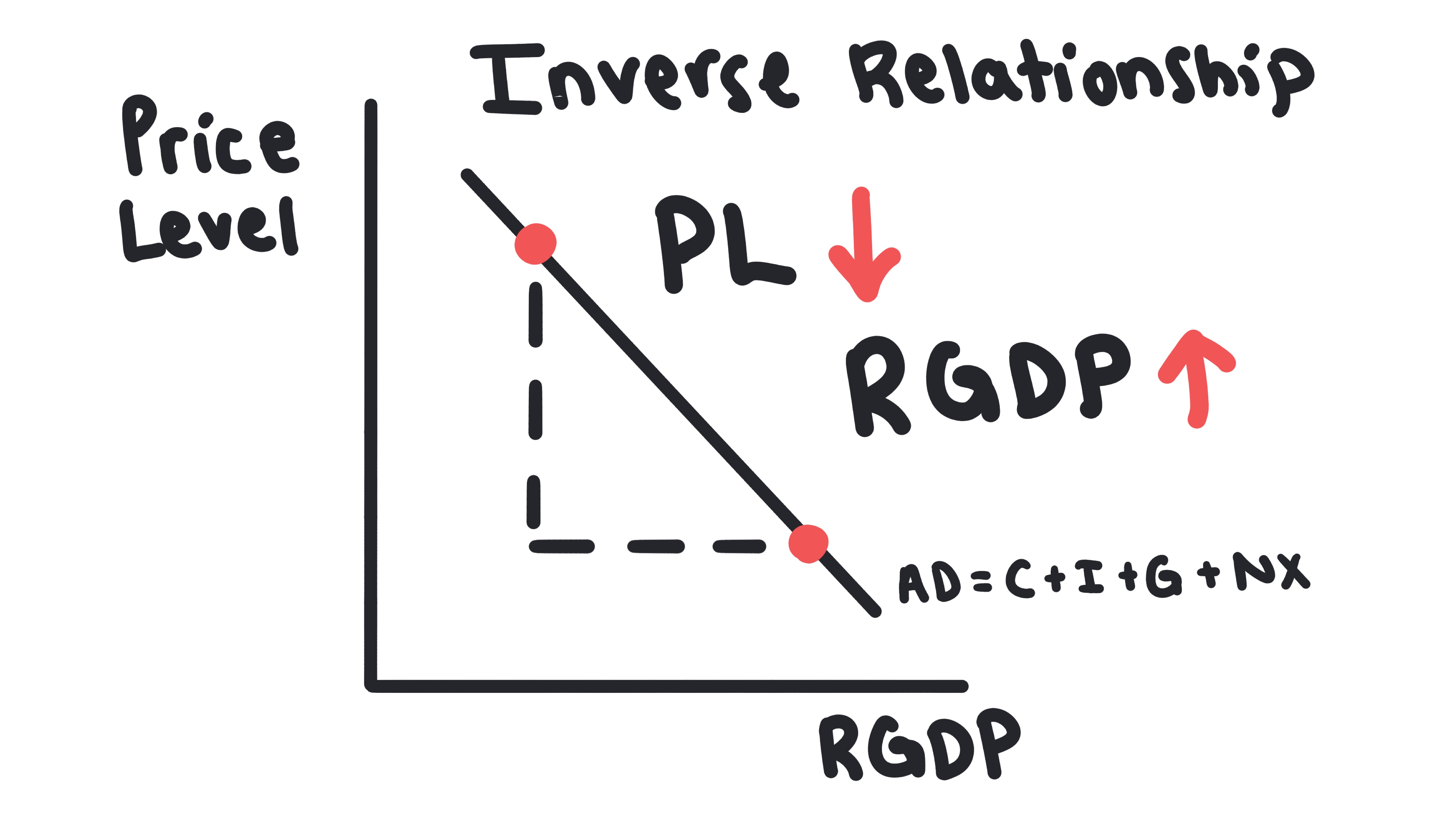
Inverse Relationship between Price Level and AD
The AD curve is downward sloping because as the price level goes down, the quantity of real GDP demanded goes up, and vice versa.
- •This inverse relationship is explained by three effects: the Real Wealth Effect, the Interest Rate Effect, and the Net Export Effect
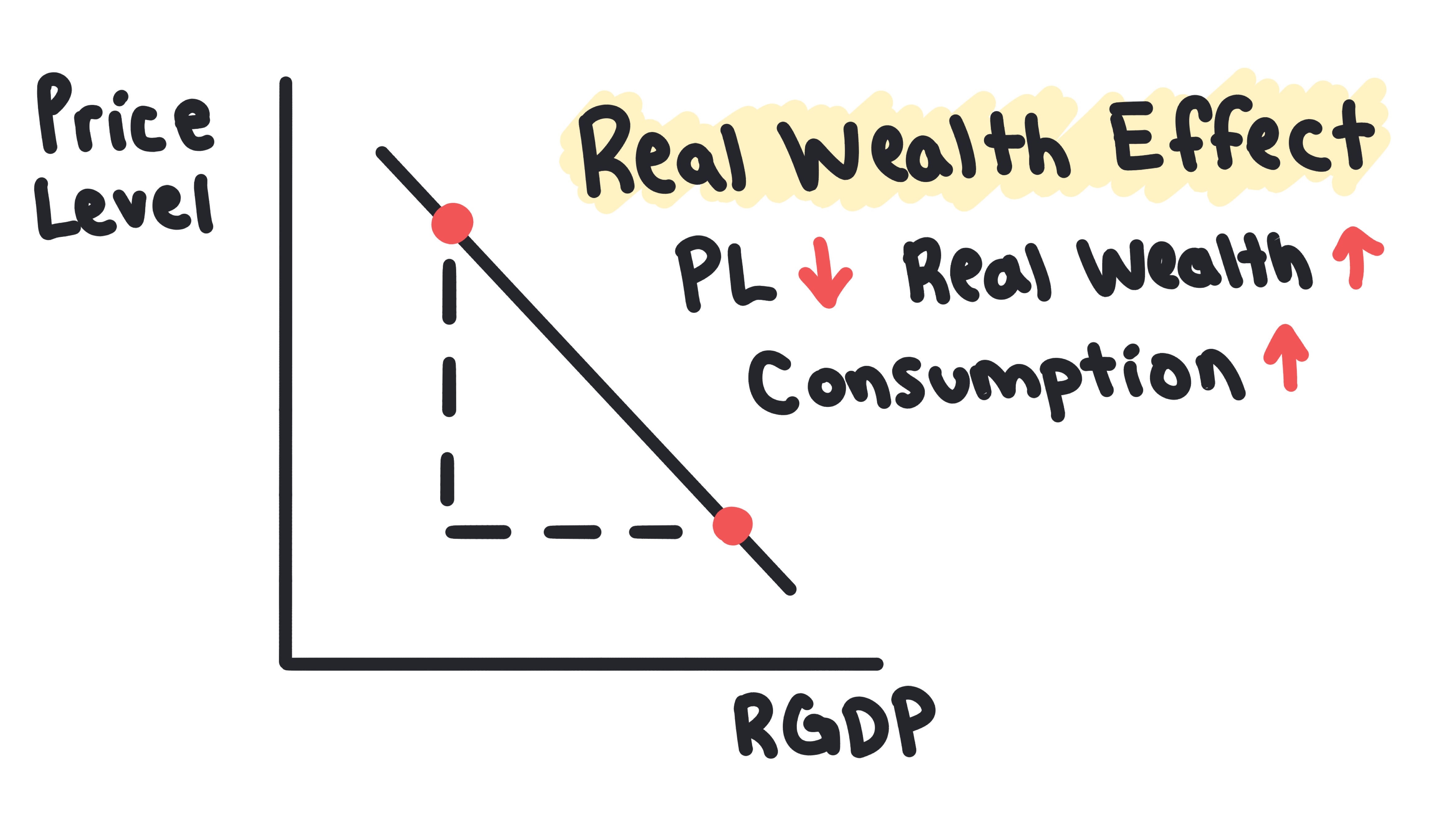
Real Wealth Effect
When the price level falls, the money you have is more valuable, making you feel wealthier and causing you to spend more.
- •Example: If you have 1000 can now buy more goods and services, making you feel wealthier. This increased purchasing power encourages you to spend more, increasing aggregate demand.
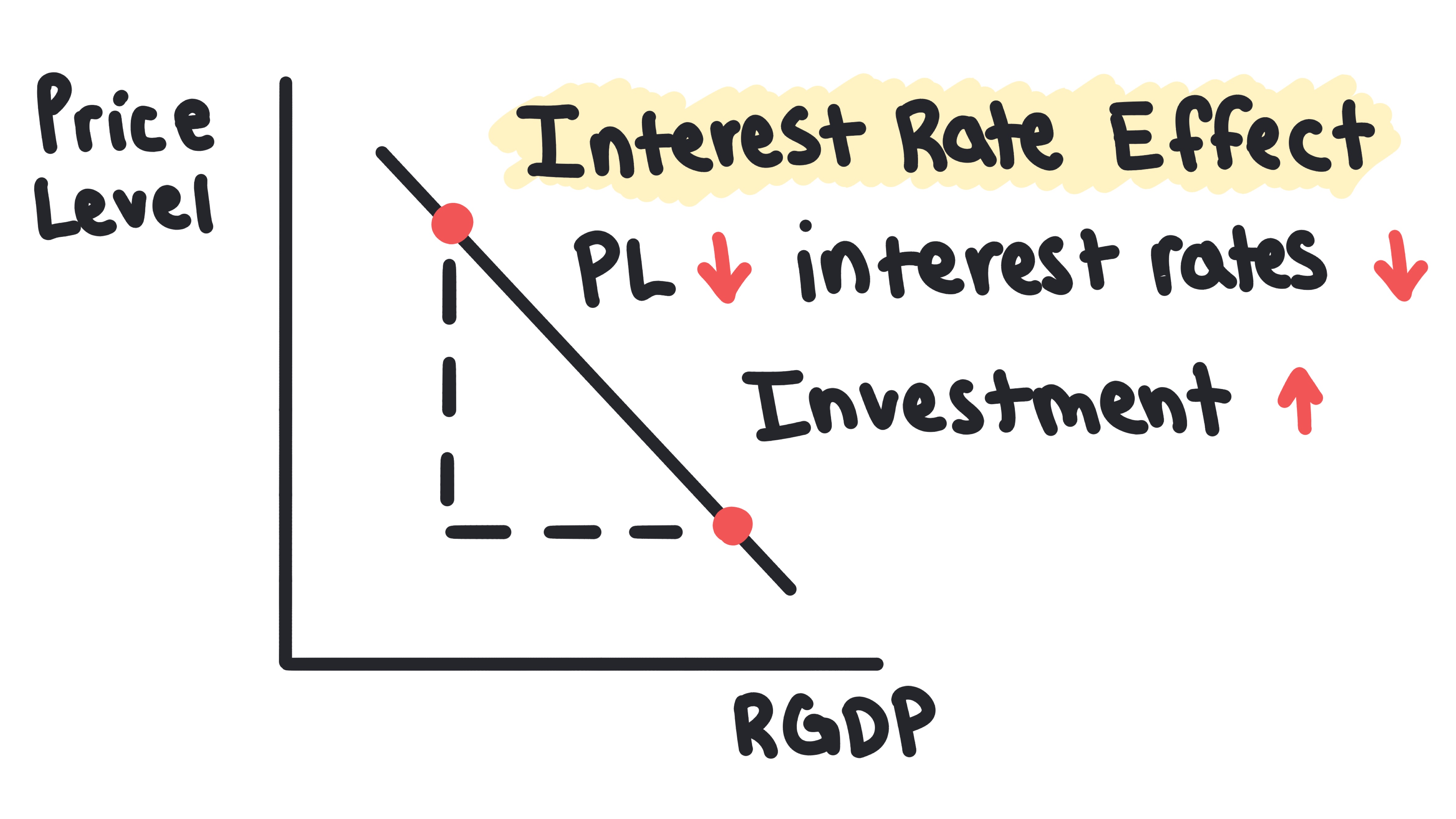
Interest Rate Effect
When the price level falls, people save more, which drives down interest rates and makes it cheaper for businesses to borrow and invest.
- •Example: When prices fall, people need less money for transactions, so they save more. This increased supply of loanable funds lowers interest rates. Lower interest rates make it cheaper for businesses to borrow money for investment projects, increasing aggregate demand.
Net Export Effect
When a country's price level falls, its goods become cheaper compared to foreign goods, which causes its net exports to go up.
- •Example: If the U.S. price level falls while prices in other countries stay the same, American goods become relatively cheaper. Foreign consumers will buy more American products, and American consumers will buy fewer foreign products, increasing U.S. net exports and aggregate demand.
Shifters of Aggregate Demand
The entire AD curve will shift when there is a change in one of the components of GDP that is not caused by a change in the price level.
- •Changes in Consumption (C): Caused by factors like consumer confidence. If fears of a recession cause consumers to lose confidence, they spend less, shifting AD to the left.
- •Changes in Investment (I): Caused by factors like business confidence. If businesses lose confidence, they invest less, shifting AD to the left.
- •Changes in Government Spending (G): Caused by direct government action. If the government passes a new spending bill, G increases, shifting AD to the right.
- •Changes in Net Exports (NX): Caused by factors like the economic health of trading partners. If a key trading partner falls into a recession, they will buy fewer of our goods, causing our net exports to fall and shifting AD to the left.
Whiteboards
Practice MCQs
Test your understanding of 3.1
Which of the following events would most likely cause the aggregate demand curve to shift to the right?
3.2 - Multipliers
Multipliers
Learn about the spending multiplier, the tax multiplier, and the affect of changes in government spending and taxes on the economy.
Key Terms & Definitions
Multiplier Effect
The ripple effect in which an initial change in spending leads to a larger total change in GDP.
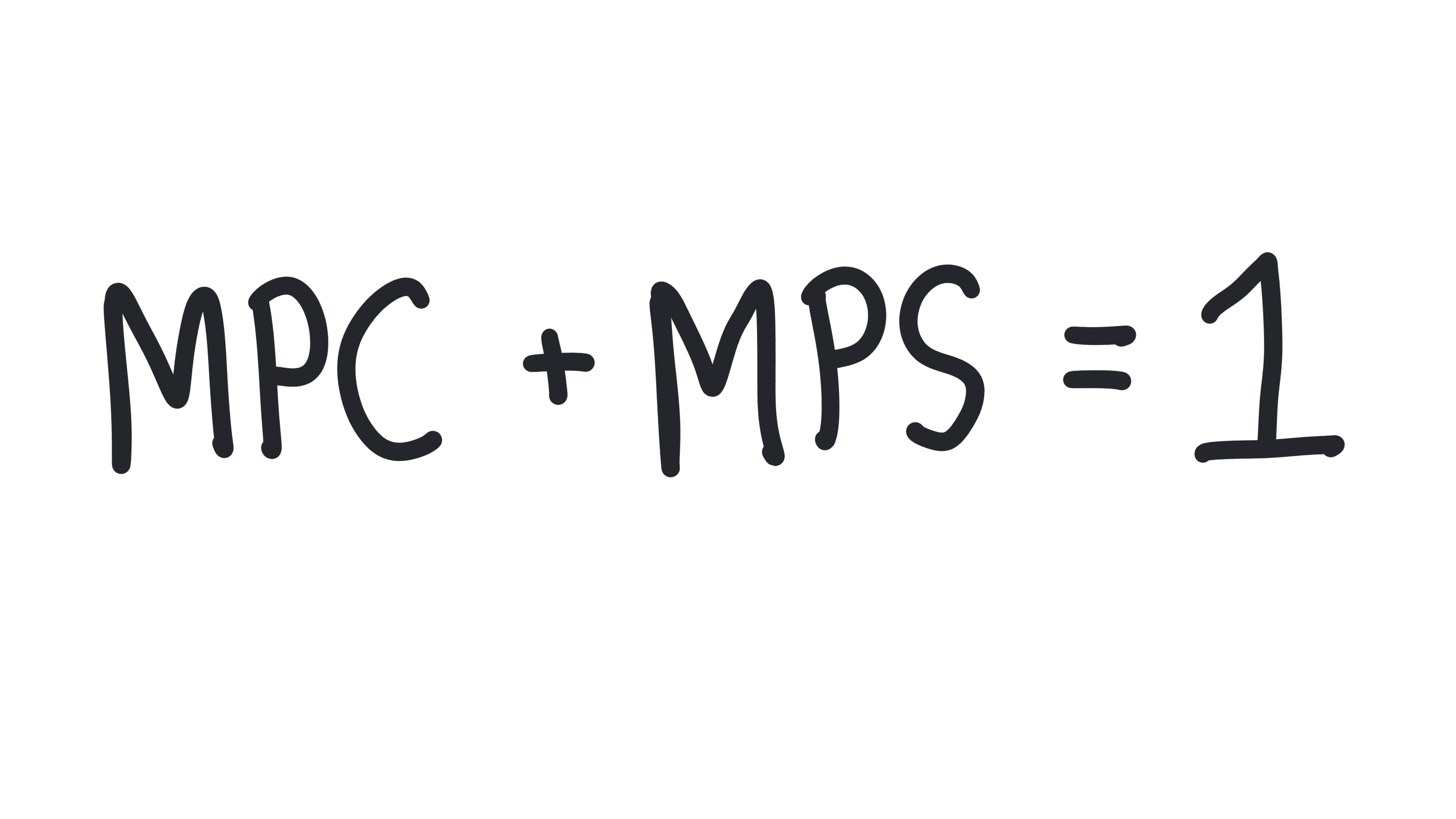
- •The size of the multiplier is determined by the marginal propensity to consume (MPC) and the marginal propensity to save (MPS)
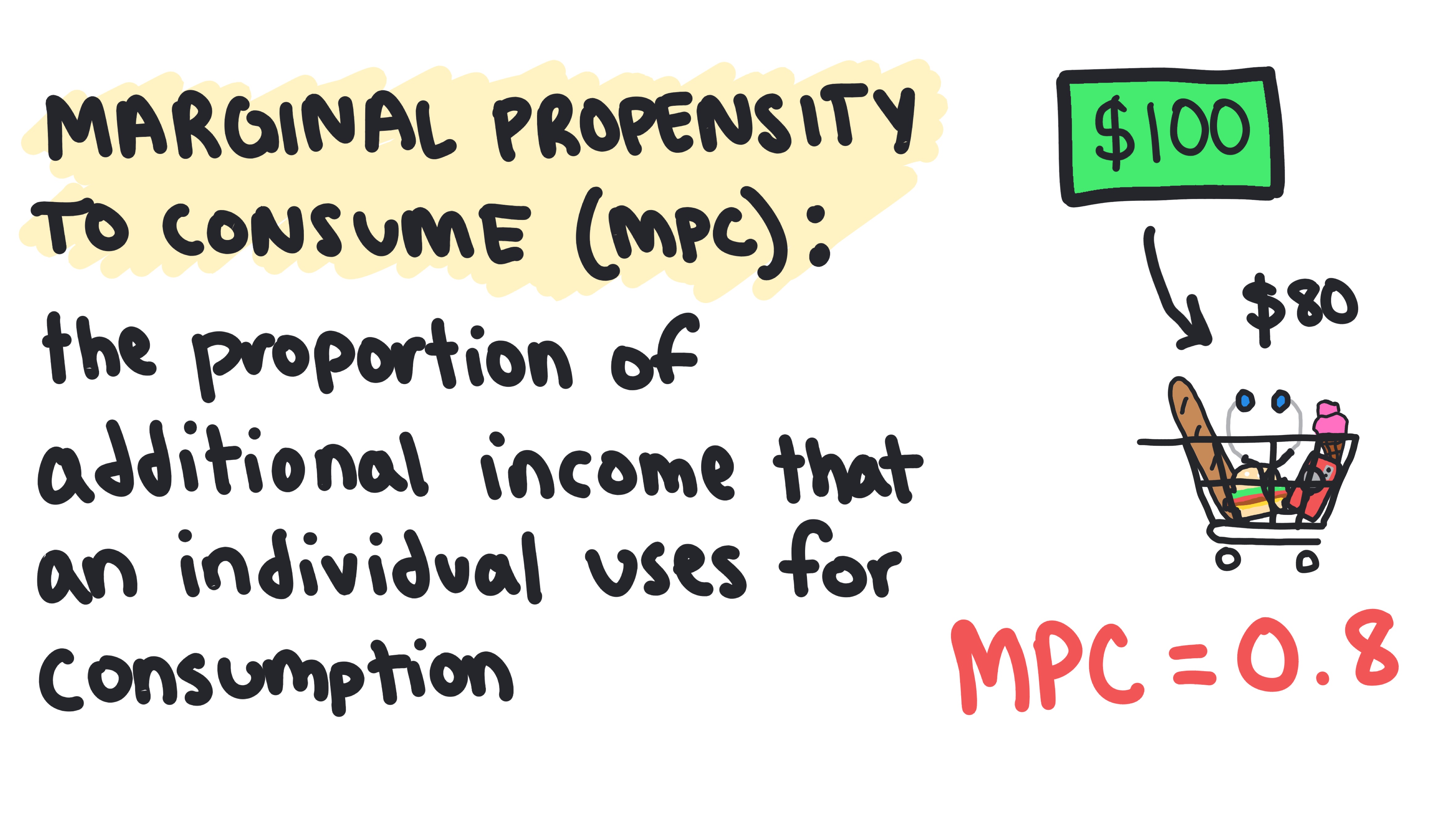
Marginal Propensity to Consume (MPC)
The fraction of any extra income that a household spends.
- •Example: If you get a 80, your MPC is 0.8.
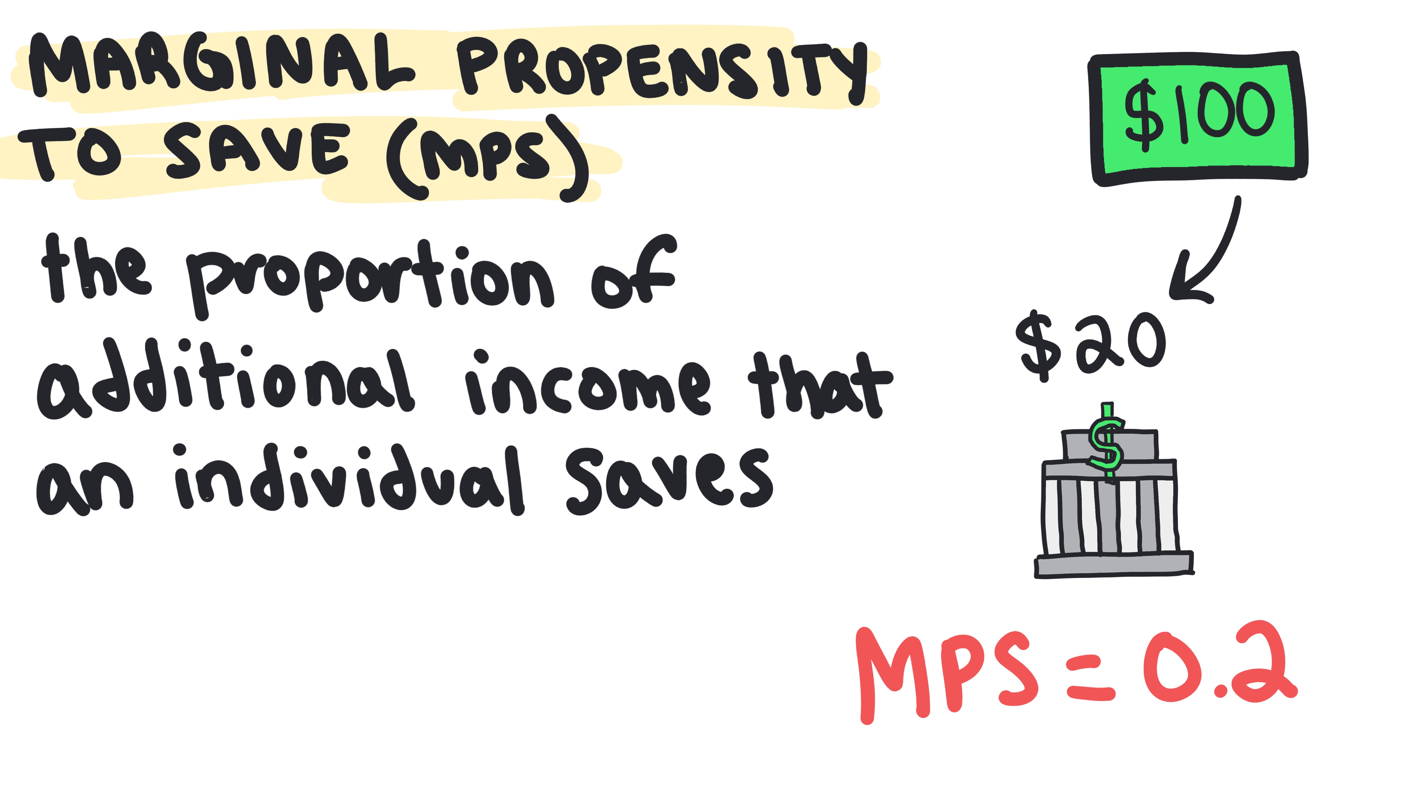
Marginal Propensity to Save (MPS)
The fraction of any extra income that a household saves.
- •Example: If you spend 100 bonus, you save $20, so your MPS is 0.2.
Spending Multiplier
A value that tells us the total change in GDP that will result from an initial change in spending.
- •Formula: 1 / MPS
Tax Multiplier
The multiplier that applies to a change in taxes.
- •Formula: -MPC / MPS
- •Note: The negative sign indicates that a decrease in taxes will increase GDP, and an increase in taxes will decrease GDP.
- •Easy trick: tax multiplier is always one less than the spending multiplier
Calculating Maximum GDP Change
Using a multiplier to find the total potential change in GDP.
- •For spending: Initial Change in Spending × Spending Multiplier
- •For taxes: Initial Change in Taxes × Tax Multiplier
Whiteboards
Practice MCQs
Test your understanding of 3.2
If the marginal propensity to save (MPS) is 0.2, and the government increases spending by $100 billion with no change in taxes, what is the maximum possible change in real GDP?
3.3 - Short-Run Aggregate Supply (SRAS)
Short-Run Aggregate Supply
Learn about the components of short-run aggregate supply, the relationship between short-run aggregate supply and the price level, and the impact of changes in short-run aggregate supply on the economy.
Key Terms & Definitions
Short-Run Aggregate Supply (SRAS)
Shows the direct relationship between the overall price level and the quantity of output that firms produce in the short run.
- •It is upward-sloping due to sticky wages
Sticky Wages
The main reason the SRAS curve slopes upward. In the short run, wages don’t change quickly, often due to contracts.
- •If I produce and sell wooden tables and the price of my tables rises while my workers wages remain "stuck," my profits go up, creating an incentive to produce more.
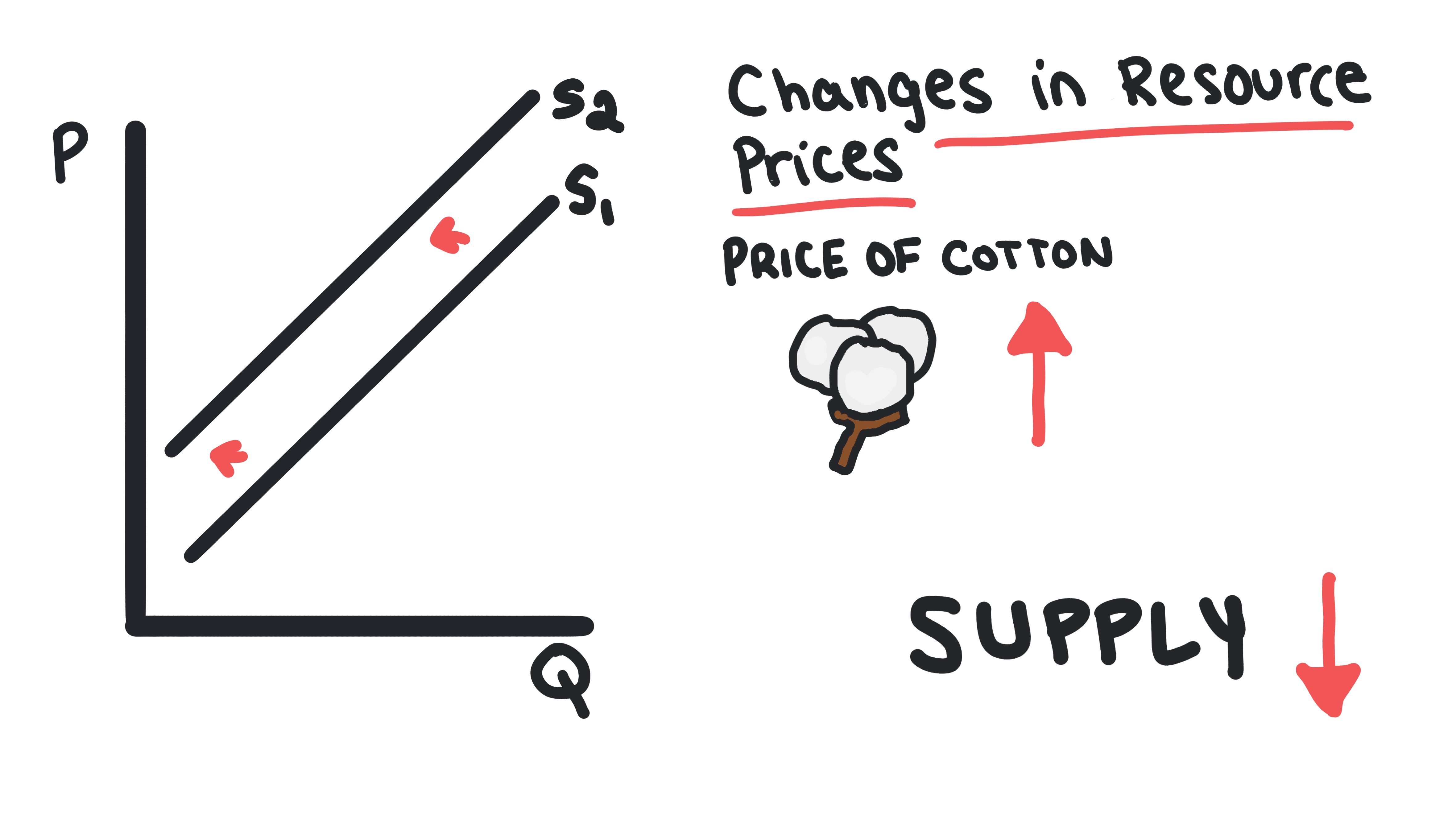
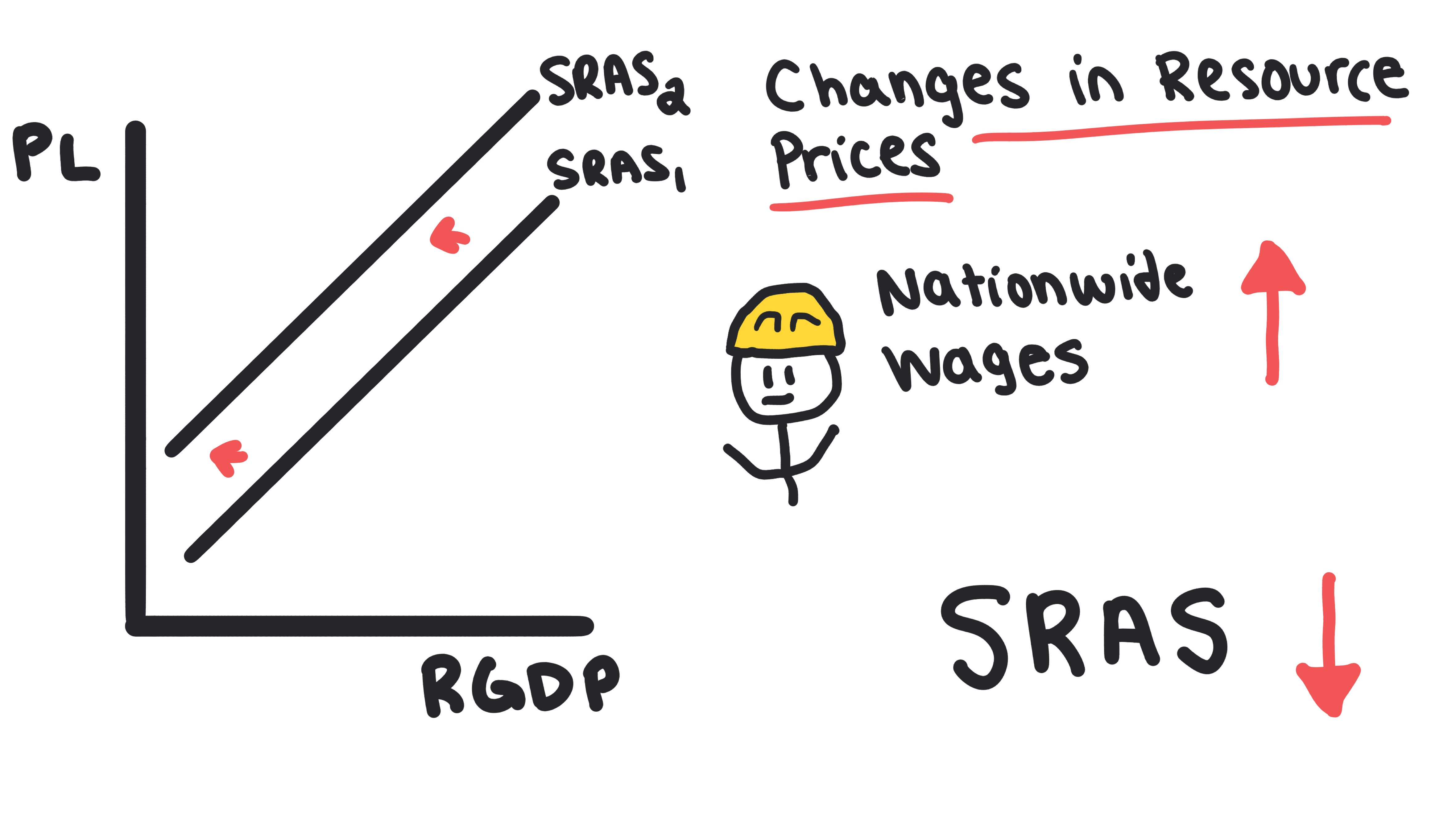
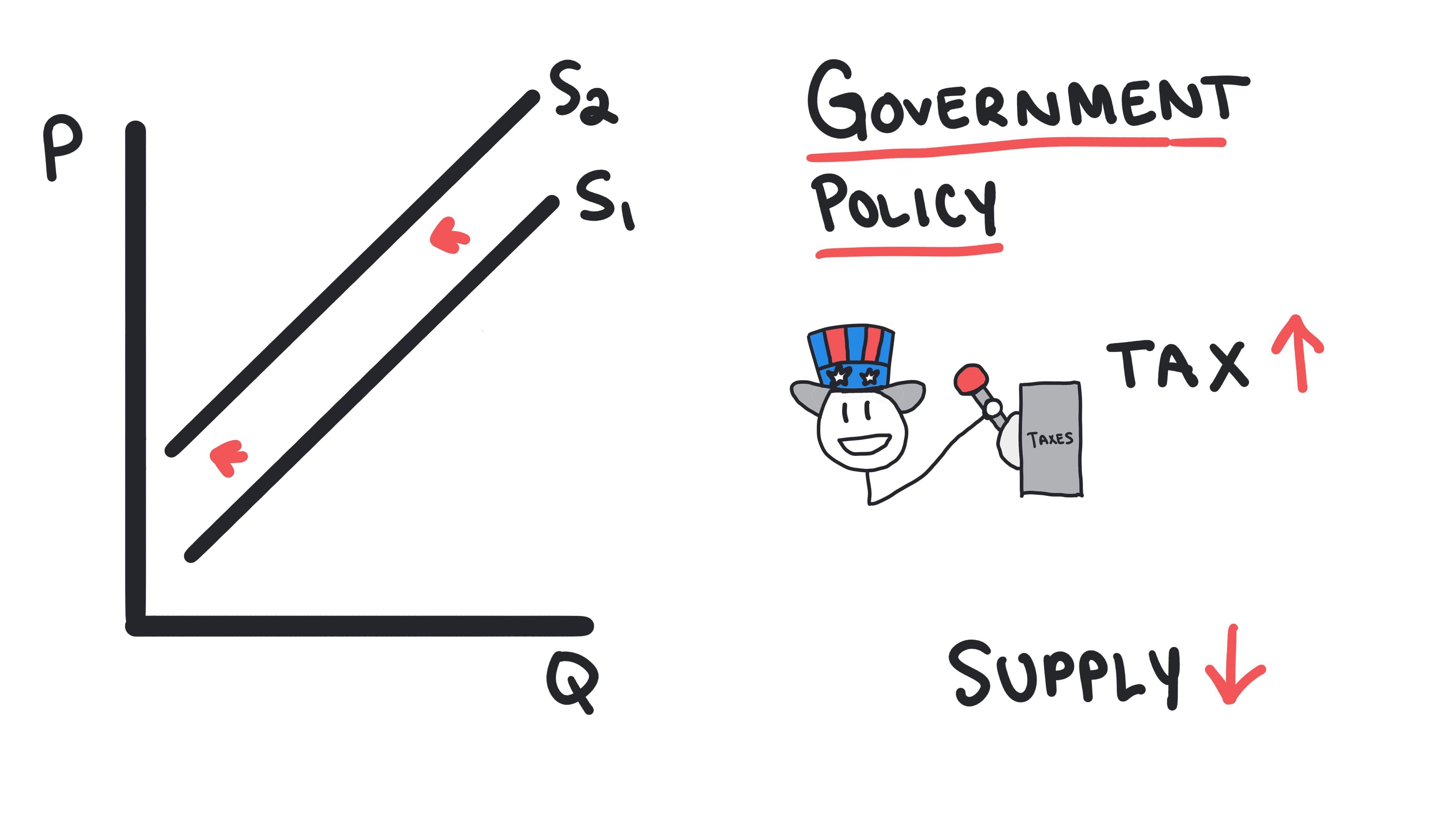
Shifters of SRAS
Non-price factors that cause the entire SRAS curve to shift, typically related to widespread changes in the costs of production.
- •Changes in resource prices (e.g., a nationwide increase in wages or oil prices)
- •Changes in government policy (e.g., business taxes or subsidies)
- •Widespread changes in technology and productivity
- •Changes in producers’ expectations about future prices
Whiteboards
Practice MCQs
Test your understanding of 3.3
Suppose there is a significant increase in the internationally traded price of energy, a major input for production in Country X. How would this likely affect the short-run aggregate supply (SRAS) and the price level in Country X?
3.4 - Long-Run Aggregate Supply (LRAS)
Long-Run Aggregate Supply
Learn about the components of long-run aggregate supply, the (lack of a) relationship between long-run aggregate supply and the price level, and the causes of changes to the LRAS curve.
Key Terms & Definitions
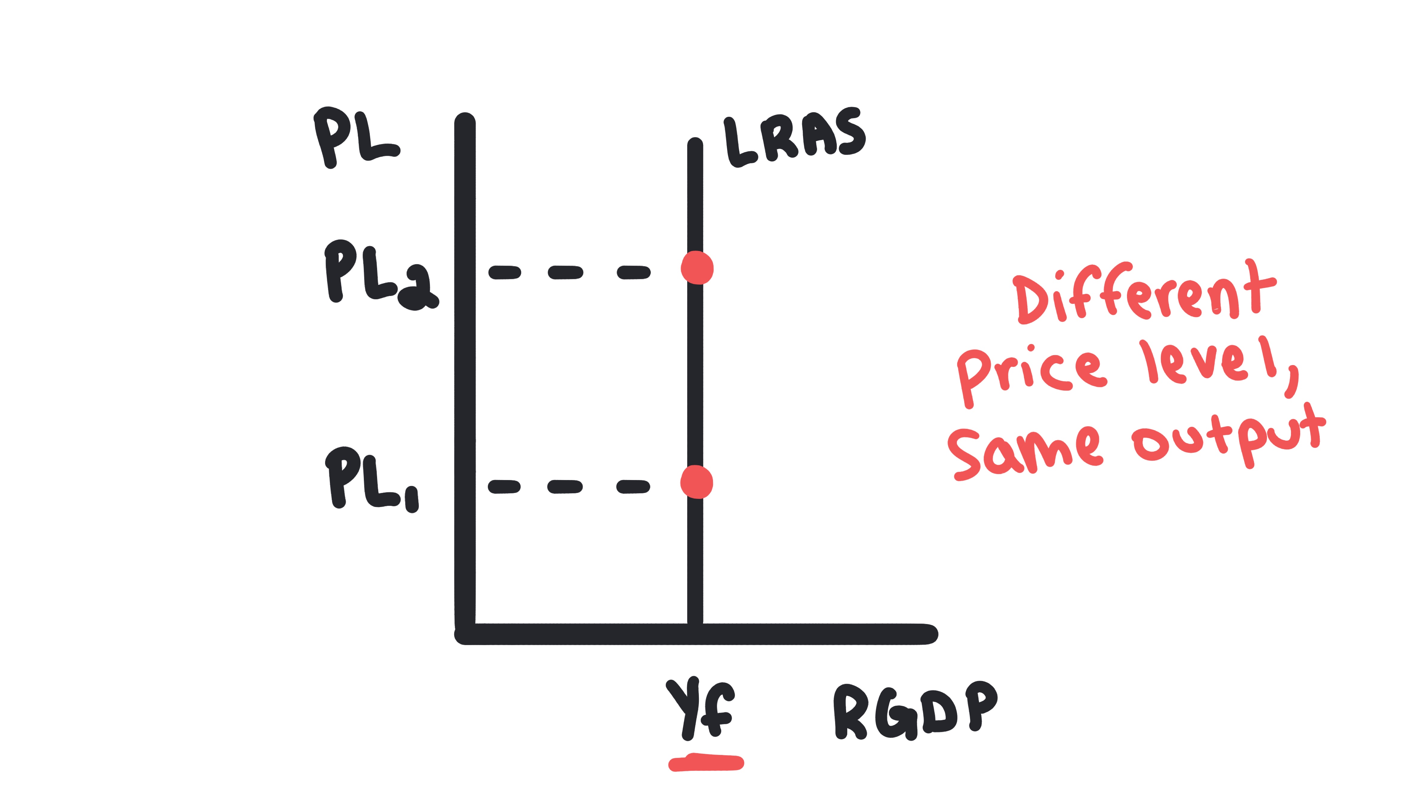
Long-Run Aggregate Supply (LRAS)
Shows the total amount of production possible for an economy when it’s using all of its resources efficiently.
- •It is a vertical line at the economy’s full-employment output level (Yf).
- •This means there is no relationship between the price level and the quantity of output that firms produce in the long run.
Full-Employment Output (Yf)
The level of output an economy can produce when it is using all of its resources efficiently; also known as potential output.
Factors of Production
The resources that determine a country’s potential output and the position of the LRAS curve.
- •Includes resources like land, labor, and capital, as well as the level of technology.
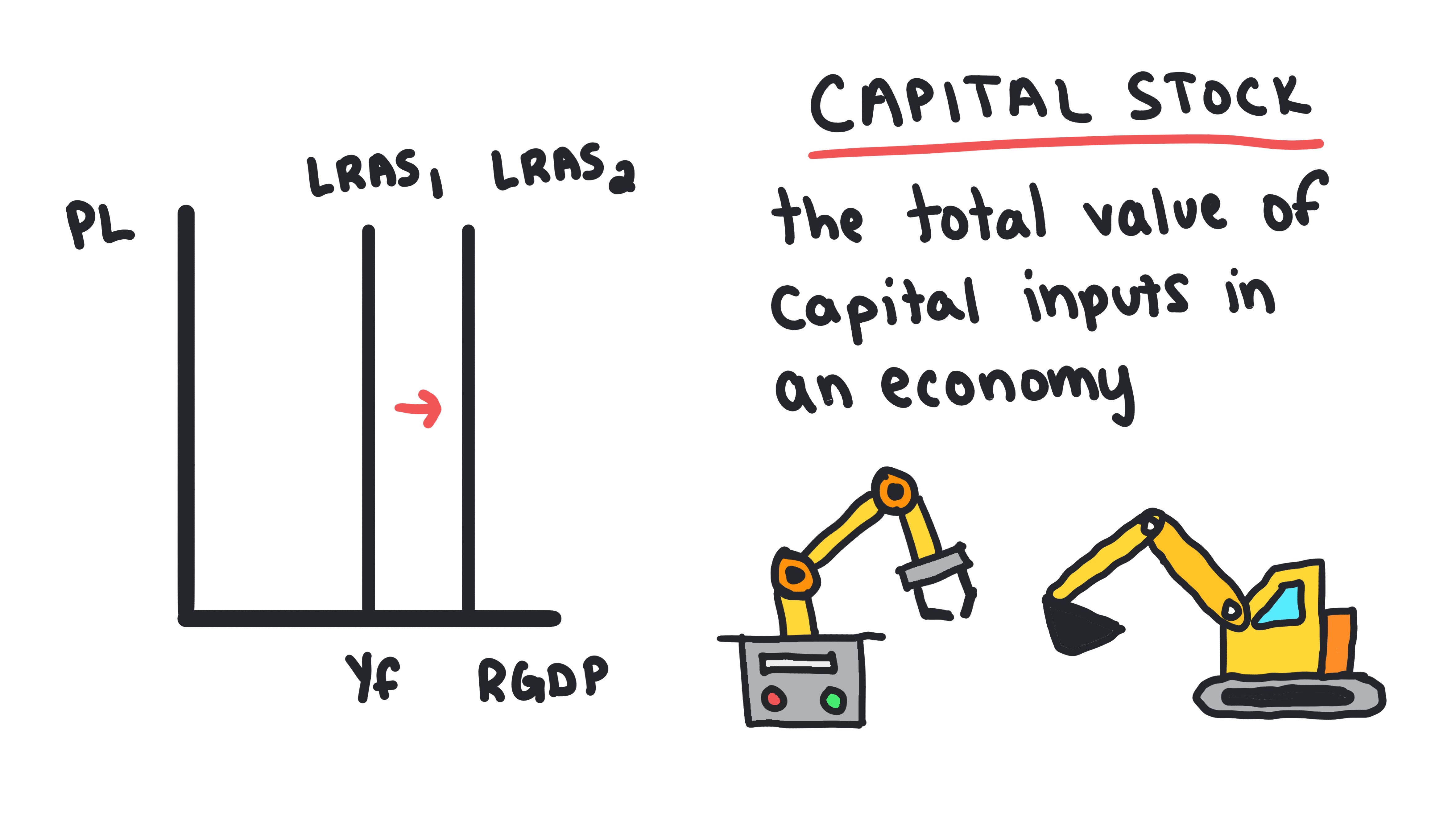
Shifters of LRAS
Factors that change a country’s productive capacity, which shifts the entire LRAS curve.
- •An increase in the capital stock or human capital causes a rightward shift
- •Discovery of new natural resources causes a rightward shift
- •A decrease in the workforce or destruction of infrastructure causes a leftward shift
Whiteboards
Practice MCQs
Test your understanding of 3.4
Refer to the graph below. A rightward shift of the Long-Run Aggregate Supply (LRAS) curve from LRAS1 to LRAS2 is best explained by:

3.5 - Equilibrium in the Aggregate Demand - Aggregate Supply (AD-AS) Model
Equilibrium in the AD-AS Model
Learn about the full AD-AS model, the concept of short-run equilibrium, long-run equilibrium, and output gaps.
Key Terms & Definitions
Short-Run Equilibrium
Occurs where the AD curve and the SRAS curve intersect. An economy will always be in a state of short-run equilibrium.
Long-Run Equilibrium
A special case where the AD, SRAS, and LRAS curves all intersect at the same point, meaning current output is equal to the country’s potential output.
Recessionary Gap
Occurs when the short-run equilibrium is to the left of the LRAS curve.
- •Actual output is less than potential output
- •Unemployment rate is greater than the natural rate
Inflationary Gap
Occurs when the short-run equilibrium is to the right of the LRAS curve.
- •Actual output is greater than potential output
- •Unemployment rate is less than the natural rate
Whiteboards


Practice MCQs
Test your understanding of 3.5
An economy's actual real GDP is currently $500 billion, while its potential real GDP (full employment output) is estimated to be $550 billion. Based on this information, which of the following is most likely true regarding the unemployment rate?
3.6 - Changes in the AD-AS Model in the Short Run
Changes in Equilibrium in the AD-AS Model
Learn about how shifts of the AD curve and SRAS curve change the equilibrium in the AD-AS model.
Key Terms & Definitions
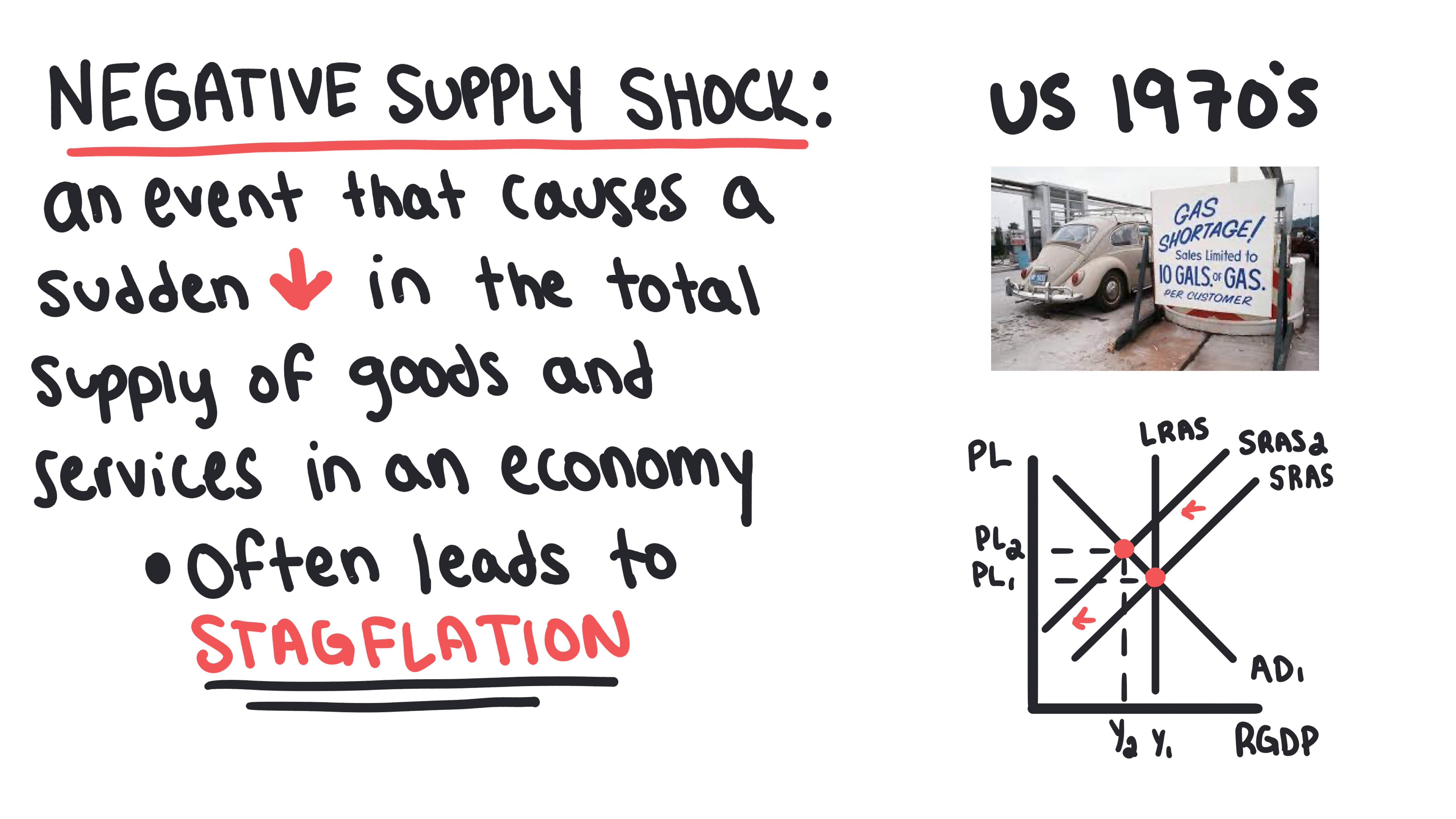
Negative Supply Shock
A sudden event that makes production more difficult or expensive across the economy, such as a sharp rise in the price of oil. It shifts the SRAS curve to the left.
- •Results in a decrease in output, an increase in the price level, and an increase in unemployment
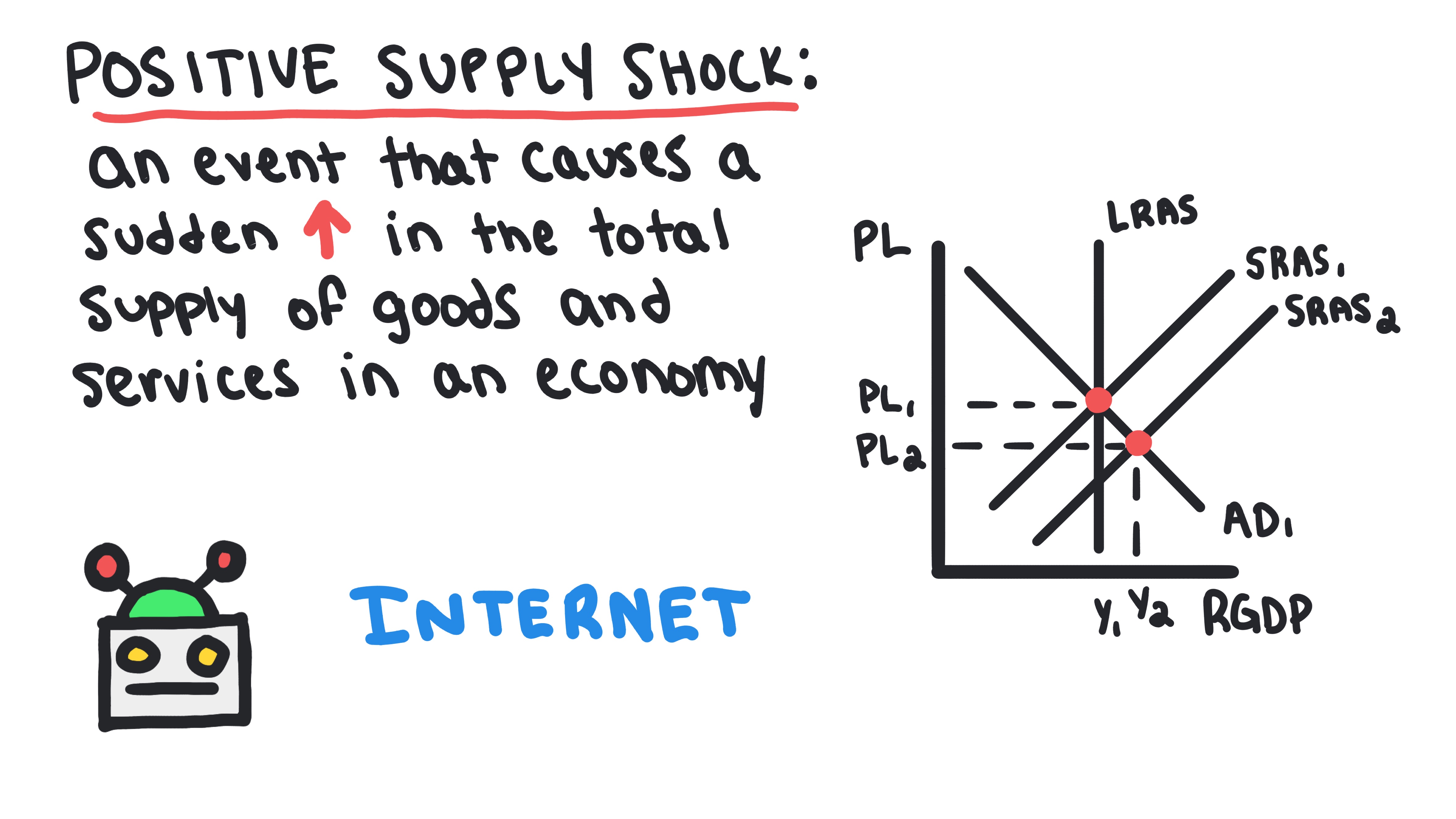
Positive Supply Shock
A sudden event that makes production easier or cheaper, such as a major technological breakthrough. It shifts the SRAS curve to the right.
- •Results in an increase in output, a decrease in the price level, and a decrease in unemployment
Stagflation
A situation, often caused by a negative supply shock, where the economy experiences both higher unemployment and a higher price level.
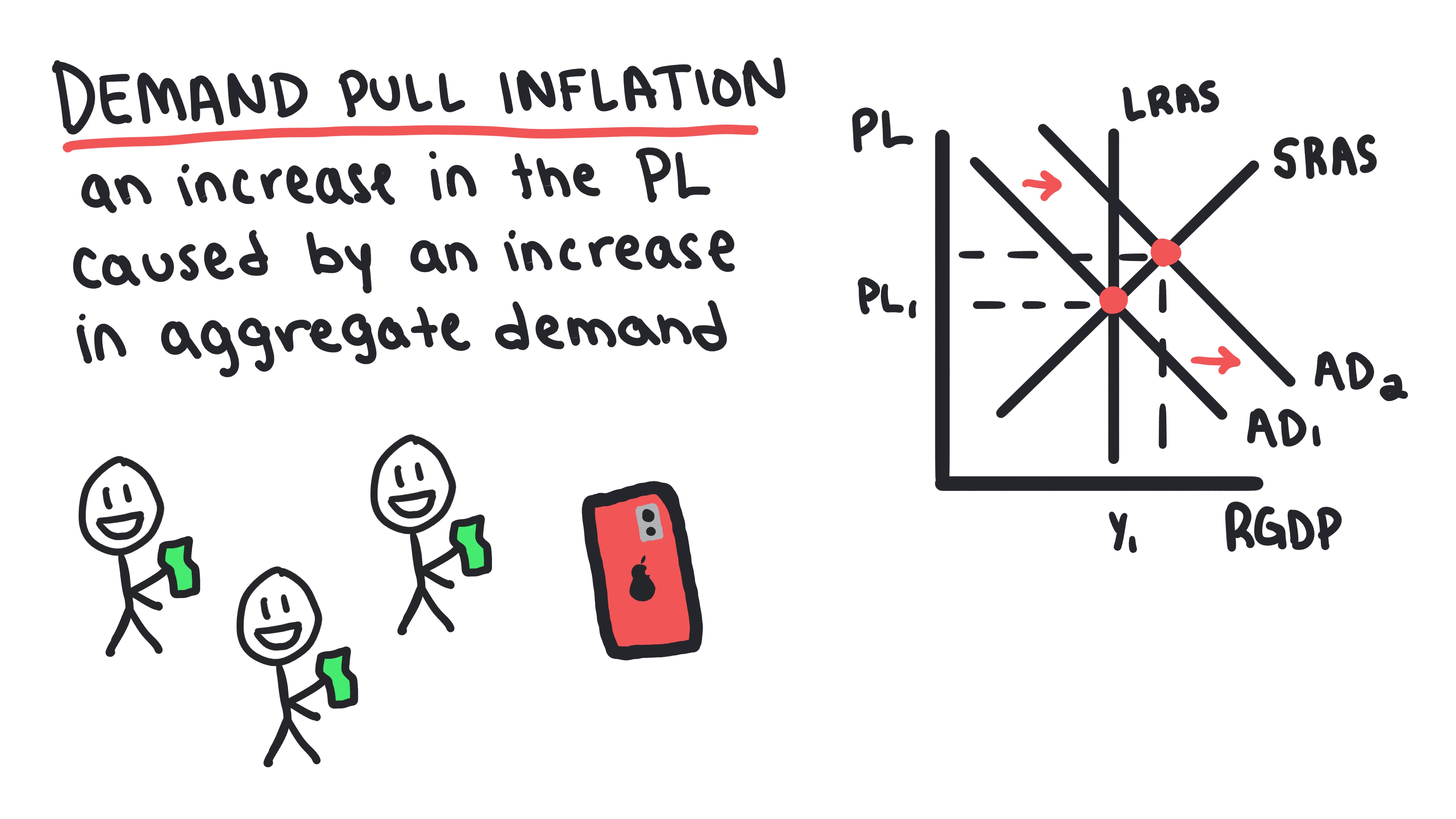
Demand-Pull Inflation
A rise in the price level caused by an increase in aggregate demand.
- •Can be thought of as "too much money chasing too few goods."
Cost-Push Inflation
A rise in the price level caused by a decrease in short-run aggregate supply, often due to higher input costs.
Whiteboards
Practice MCQs
Test your understanding of 3.6
Assume an economy is initially in long-run equilibrium. The government then significantly increases its spending on infrastructure projects without changing taxes. In the short run, what is the most likely impact on the price level and real GDP?
3.7 - Long-Run Self-Adjustment
Fiscal Policy & Long-Run Self-Adjustment
Learn about how an economy returns to long-run equilibrium from an output gap.
Key Terms & Definitions
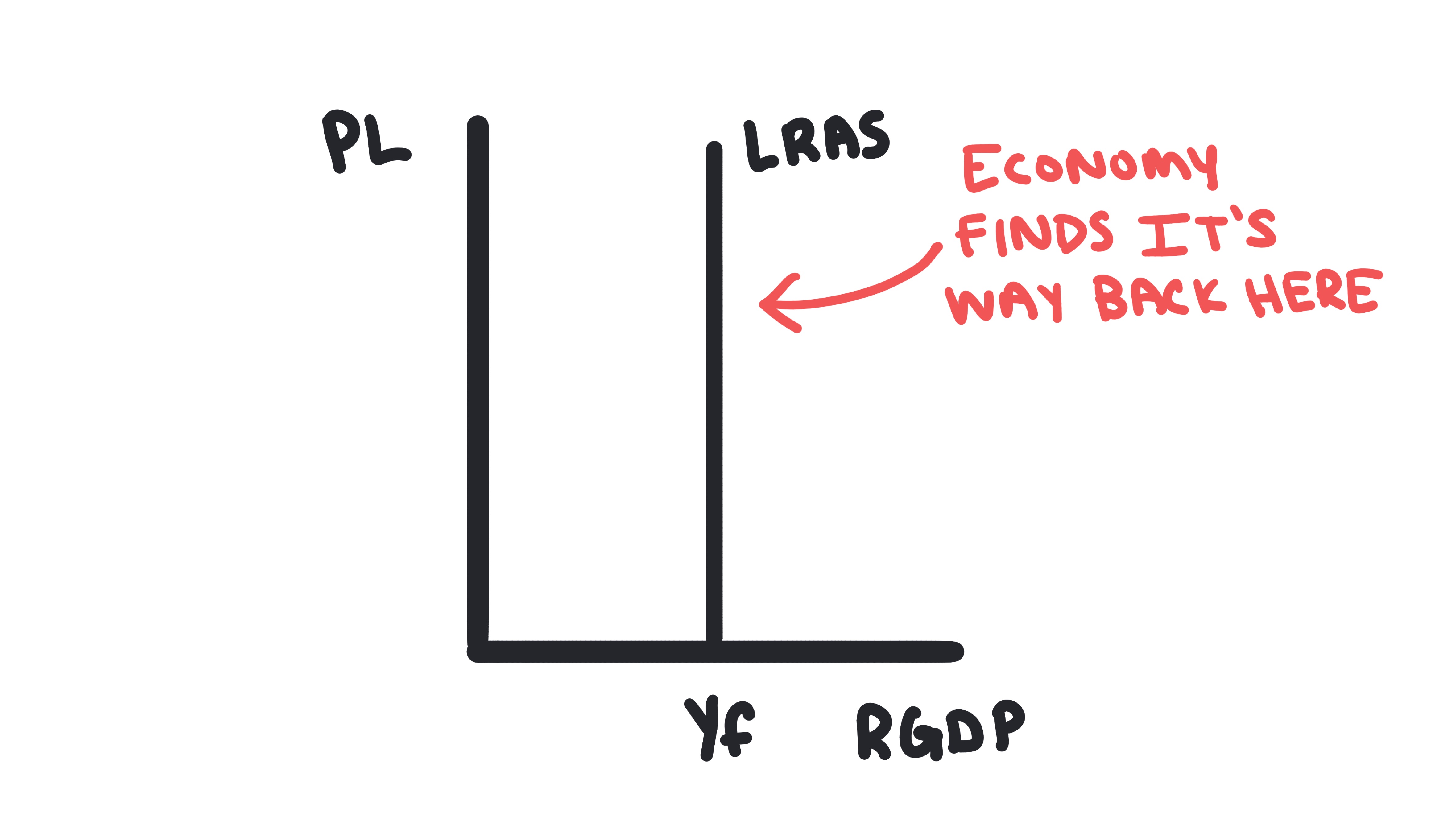
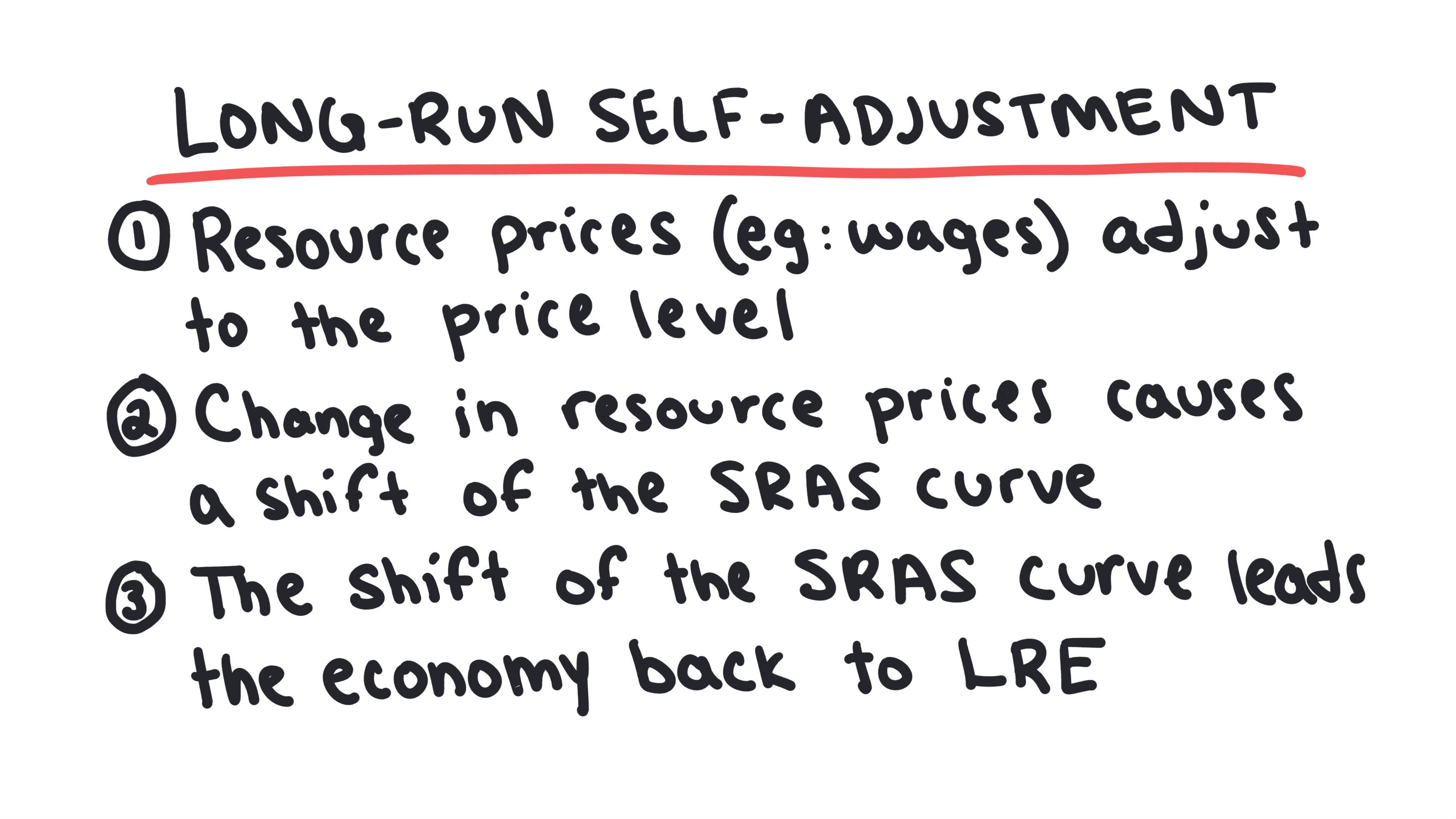
Long-Run Self-Adjustment
The process through which an economy gets out of an output gap and back to long-run equilibrium on its own, without government action.
- •Driven by changes in resource prices, like wages, which shift the SRAS curve.
Self-Adjustment from a Recessionary Gap
The process by which an economy naturally returns to long-run equilibrium from a recessionary gap.
- •High unemployment causes nominal wages to fall
- •Lower wages shift the SRAS curve to the right
- •Economy returns to full-employment output at a lower price level
Self-Adjustment from an Inflationary Gap
The process by which an economy naturally returns to long-run equilibrium from an inflationary gap.
- •Low unemployment causes wages to rise
- •Higher wages shift the SRAS curve to the left
- •Economy returns to full-employment output at a higher price level
Long-Run Impact of Self-Adjustment
The final outcome for an economy after it moves into an output gap and then self-adjusts.
- •In the long run, output returns to full-employment level
- •Price level changes to bring the economy back to equilibrium
Whiteboards
Practice MCQs
Test your understanding of 3.7
An economy's actual real GDP is currently $500 billion, while its potential real GDP (full employment output) is estimated to be $550 billion. Based on this information, which of the following is most likely true regarding the unemployment rate?
3.8 - Fiscal Policy
Fiscal Policy & Long-Run Self-Adjustment
Learn about how an economy returns to long-run equilibrium from an output gap.
Key Terms & Definitions
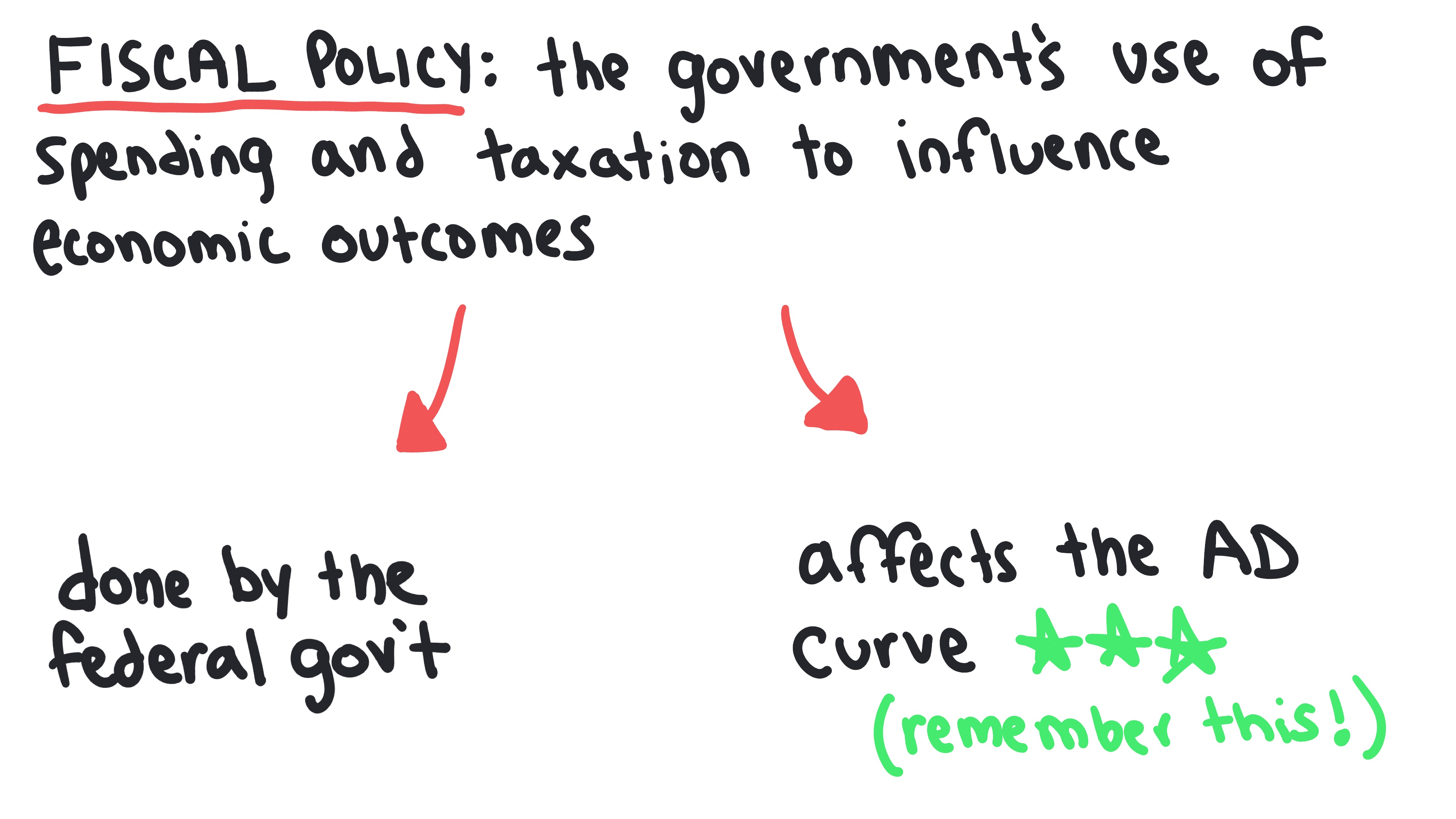
Fiscal Policy
The government’s use of spending and taxation to influence the economy.
- •Action taken by the federal government
- •Directly affects aggregate demand
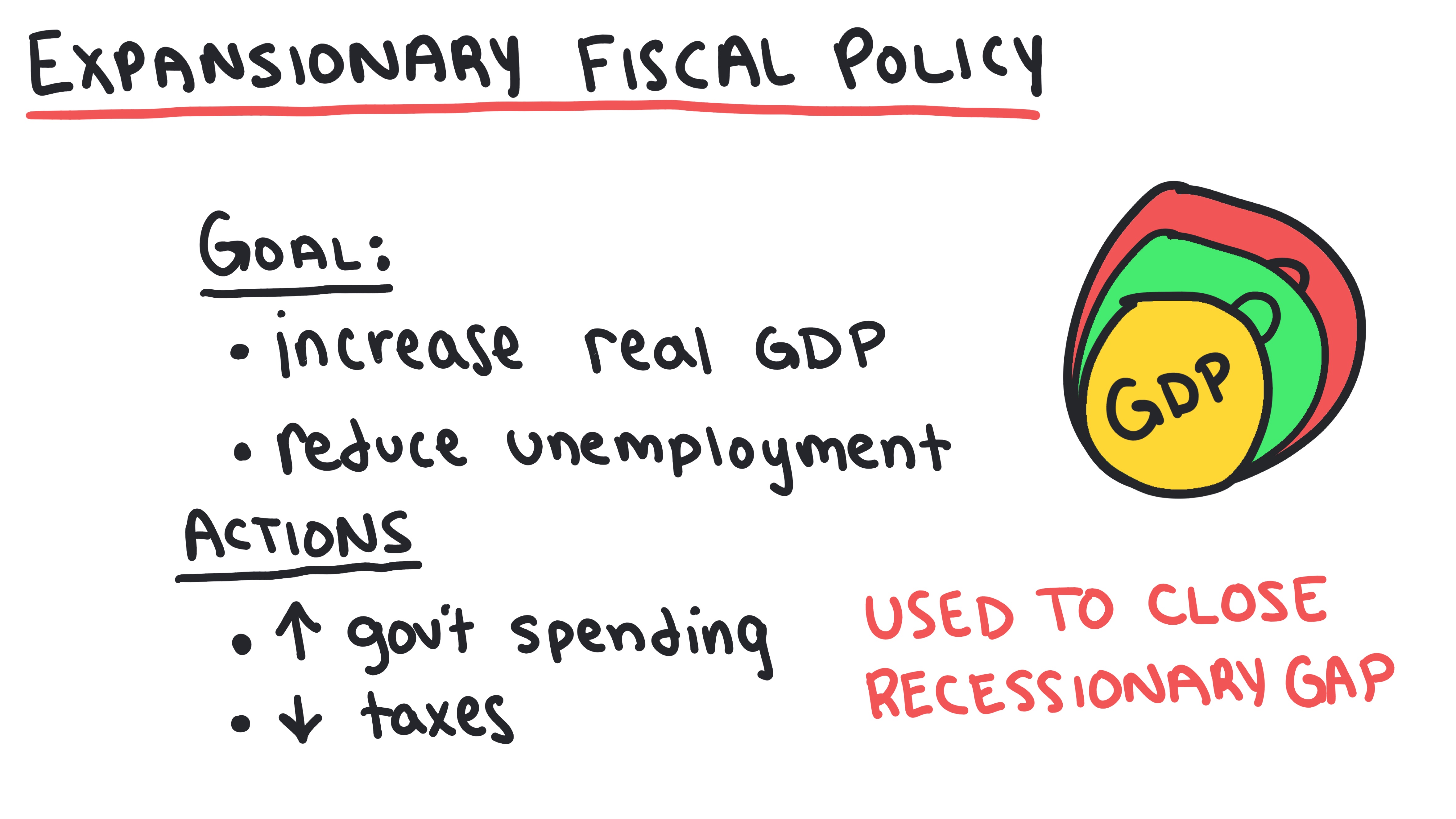
Expansionary Fiscal Policy
Policy used to stimulate the economy during a recessionary gap by increasing spending or decreasing taxes.
- •Shifts aggregate demand to the right
- •Increases the price level
- •Increases real GDP
- •Decreases unemployment
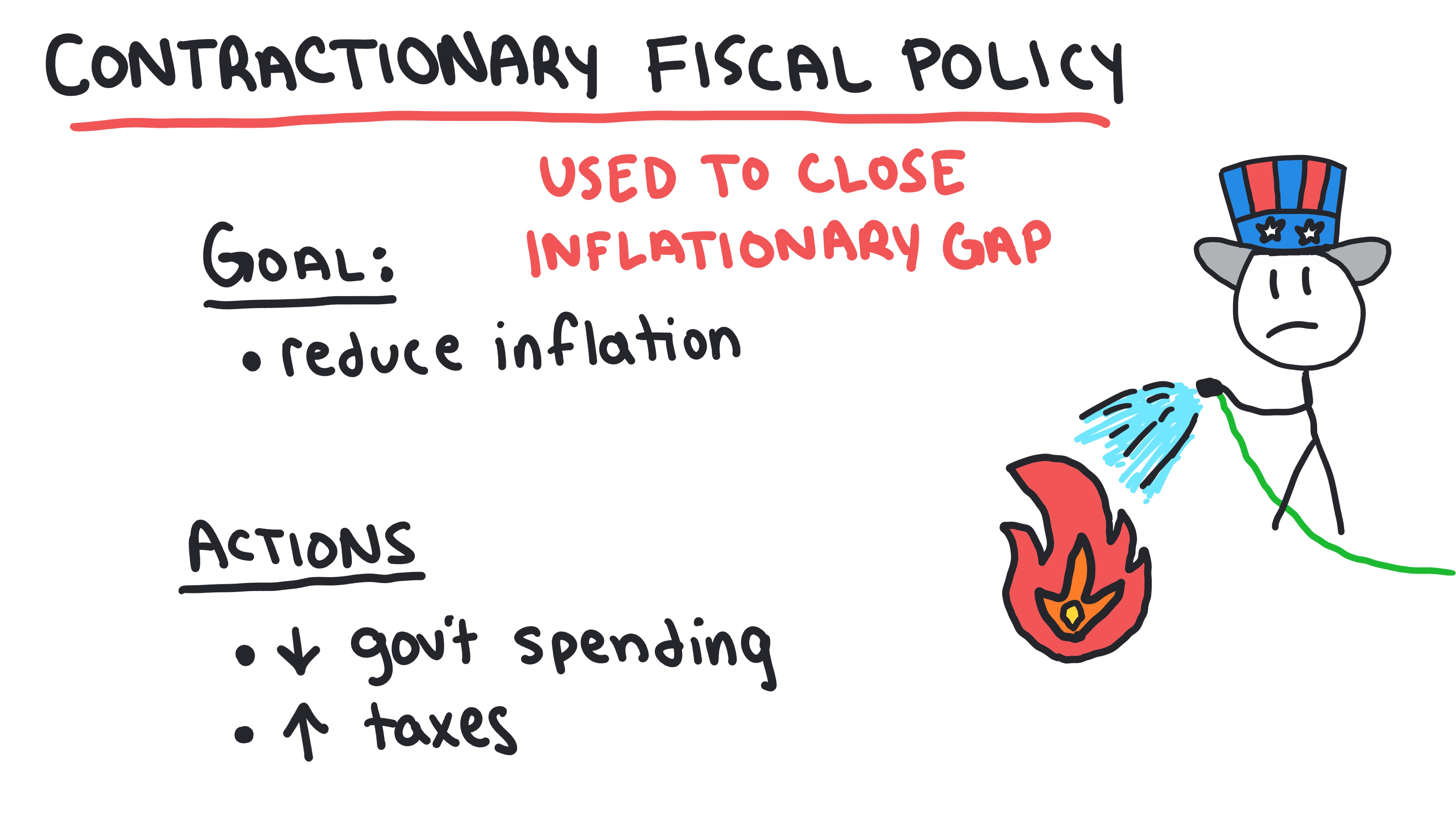
Contractionary Fiscal Policy
Policy used to slow the economy during an inflationary gap by decreasing spending or increasing taxes.
- •Shifts aggregate demand to the left
- •Decreases the price level
- •Decreases real GDP
- •Increases unemployment
Whiteboards
Practice MCQs
Test your understanding of 3.8
Assume an economy is initially in long-run equilibrium. The government then significantly increases its spending on infrastructure projects without changing taxes. In the short run, what is the most likely impact on the price level and real GDP?
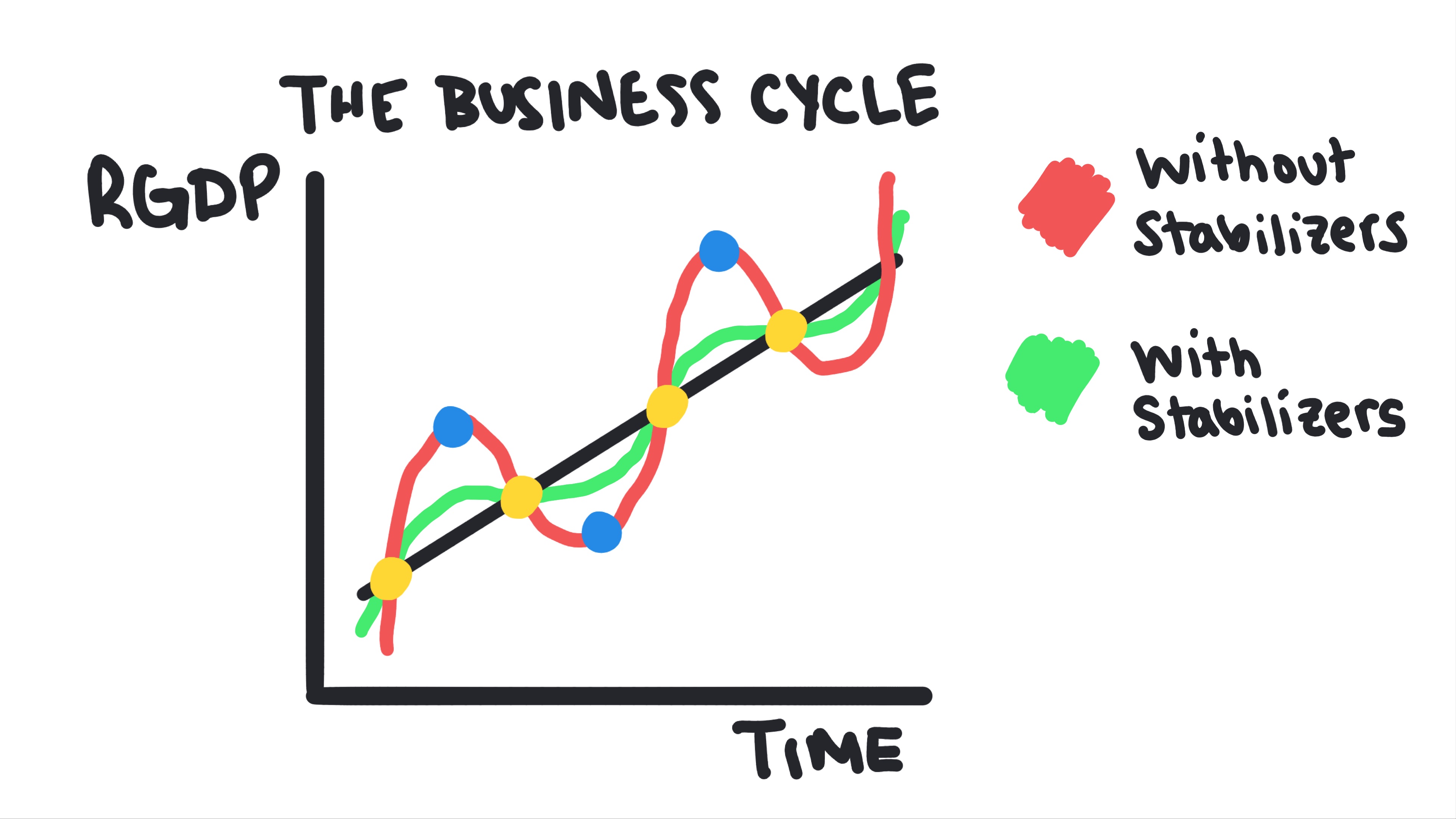
3.9 - Automatic Stabilizers
Automatic Stabilizers
Learn about how automatic stabilizers help the economy self-correct to long-run equilibrium.
Key Terms & Definitions
Discretionary Fiscal Policy
When lawmakers make explicit, deliberate changes to spending and taxes.
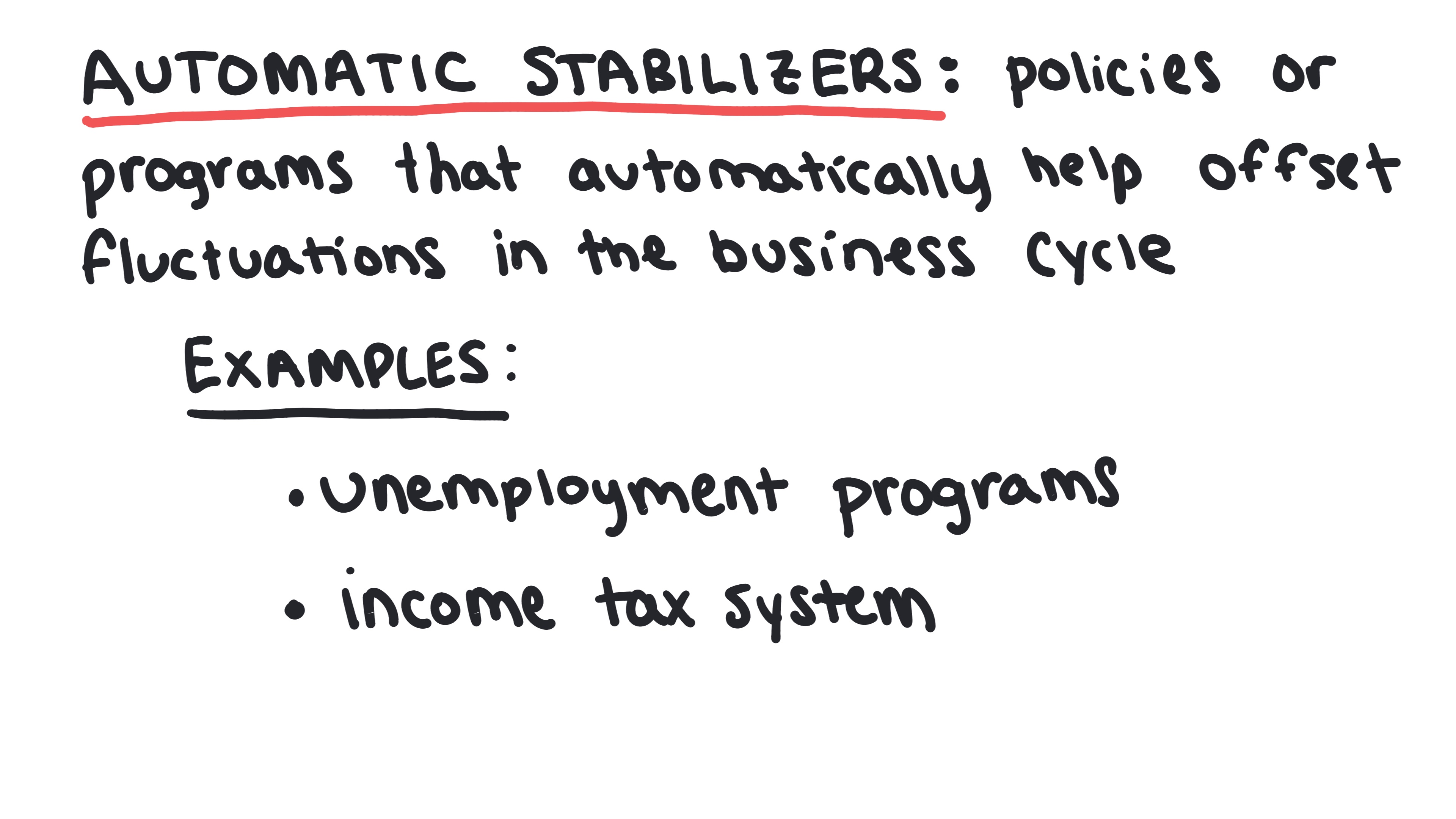
Automatic Stabilizers
Features of the tax and spending system that work to stabilize the economy automatically, without any new action from lawmakers.
- •Common examples include unemployment benefits and the income tax system
Whiteboards
Practice MCQs
Test your understanding of 3.9
During an economic expansion, the nation's progressive income tax system results in automatically higher tax revenues. This phenomenon is an example of: